1 Ulva organellar genomes retrieval and preparation

1.1 On this page

Biological insights and take-home messages are at the bottom of the page at Lesson Learnt: Section 1.3.

Here we retrieve Ulva organellar genomes;
we investigate the organellar genome availability and the gene occupancy across the retrieved genomes.

1.2 Dataset overview

1.2.1 Dataset retrieval

We included the following species 50 Ulva species, that as for 2022 where the most comprehensive list of chloroplasts and mitochondrial complete genomes published for Ulva.

Oltmassiellopsis viridis and Pseudendoclonium akinetum were used as an outgroup to root the phylogenetic tree.

Organellar genome sequences and gene models were retrieved from NCBI, and corrected where necessary.

1.2.2 Gene occupancy

The gene matrix occupancy and gene length distribution across organellar genomes included in this study are presented below. Most selected genes are present/ nearly present in all studied sequences. Based on the gene occupancy, we selected 29 genes from the mitochondrial genomes for the downstream analyses, and 70 genes from the chloroplast genomes.

# read tables
cp_mt_genes_occupancy = read.delim("./data/cp_mt_genes_occupancy.tab")

# drop last line which is uninformative
cp_mt_genes_occupancy = head(cp_mt_genes_occupancy, -1)

# format headers
colnames(cp_mt_genes_occupancy) = stringr::str_remove_all(colnames(cp_mt_genes_occupancy), ".aln.fa")
colnames(cp_mt_genes_occupancy) = stringr::str_replace_all(colnames(cp_mt_genes_occupancy), "X..Sequences", "Species")

# melt and clean
cp_mt_genes_occupancy = reshape2::melt(cp_mt_genes_occupancy)
cp_mt_genes_occupancy$organell = ifelse(
  stringr::str_detect(cp_mt_genes_occupancy$variable, "_cp_CDS_"),
  "Chloroplast",
  "Mitochondrion"
)
cp_mt_genes_occupancy$variable = stringr::str_remove_all(cp_mt_genes_occupancy$variable, "X02_cp_CDS_align.")
cp_mt_genes_occupancy$variable = stringr::str_remove_all(cp_mt_genes_occupancy$variable, "X02_mt_CDS_align.")
# set different number to assign different color to mitochondrial genes
cp_mt_genes_occupancy$value = ifelse(
  cp_mt_genes_occupancy$value == 1 & cp_mt_genes_occupancy$organell == "Mitochondrion",
  2,
  cp_mt_genes_occupancy$value
)
cp_mt_genes_occupancy$value = as.character(cp_mt_genes_occupancy$value)

# plot
p1 = ggplot(cp_mt_genes_occupancy) +
  geom_tile(aes(x = variable, y = Species, fill = value), color = "grey75") +
  scale_fill_manual(values = c("white", "#469d89", "steelblue")) +
  facet_grid(~organell, scales = "free", space = "free_x") +
  labs(x = "Genes",
       y = "Species") +
  theme(plot.title = element_text(size = 24, hjust = 0.5),
        axis.ticks.x = element_blank(),
        axis.ticks.y = element_blank(), 
        axis.text.x = element_text(angle = 90, hjust = 1, vjust = 0.5),
        legend.position = "none",
        panel.background = element_blank(),
        panel.border = element_rect(colour = "black", fill = NA),
        strip.background = element_rect(colour = "NA", fill = "NA"),
        strip.placement = "outside",
        strip.text = element_text(size = 10, angle = 0, vjust = 0.5, hjust = 0.5))
plot(p1)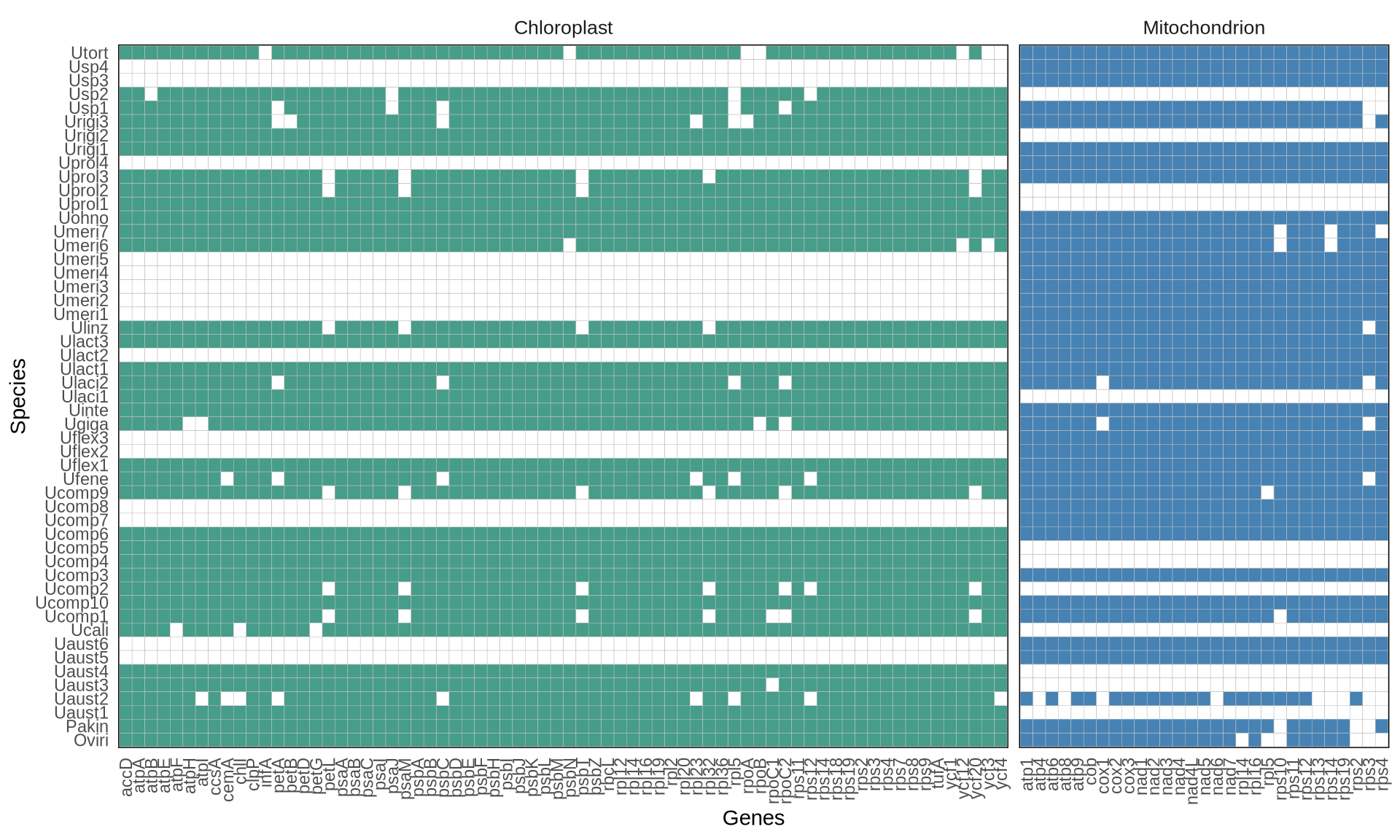

1.2.3 Gene alignments distributions

Next, we retrieved the CDS sequences and we align them. To do so, first we extract all CDSs that are longer than 200 bp from the .fasta .gff files pairs for each organellar genome.

#!/usr/bin/env bash

# get CP genes list
cut -f 9 00_cp_GenBank_RAW/*.gff \
  | sed "s/Name=//g" \
  | sed "s/ .*//g" \
  | grep "accD\|atp\|ccsA\|cemA\|chlI\|clpP\|ftsH\|infA\|pafI\|pbf1\|pet\|psa\|psb30\|psb\|rbcL\|rnl\|rns\|rpl\|rpo\|rps\|rrn5\|tufA\|ycf" \
  | sort -u \
  > cp_gene_list.lst

# extract CP fasta sequences
while read GENE; do
    for file in 00_cp_GenBank_RAW/*[0-9].fasta; do
        grep $GENE $(basename $file .fasta).cds.gff > tmp.gff;
        bedtools getfasta -fi $file -bed tmp.gff | tr ":" " ";
    done > 01_cp_CDS/$GENE.fa;
    rm tmp.gff;
done < cp_gene_list.lst


# get MT genes list
cut -f 9 00_mt_GenBank_RAW/*.gff \
  | sed "s/Name=//g" \
  | sed "s/ .*//g" \
  | sed "s/ATP/atp/g" \
  | sed "s/NAD/nad/"  \
  | grep "atp\|cob\|cox\|nad\|rpl\|rps" \
  | sort -u \
  > mt_gene_list.lst

# extract MT fasta sequences
while read GENE; do
    for file in 00_mt_GenBank_RAW/*[0-9].fasta; do
        grep $GENE $(basename $file .fasta).cds.gff > tmp.gff;
        bedtools getfasta -fi $file -bed tmp.gff | tr ":" " ";
    done > 01_mt_CDS/$GENE.fa;
    rm tmp.gff;
done < mt_gene_list.lst

We will use faTrans to translate the nucleotidic sequences to the corresponding amino-acid sequences, MAFFT to align the amino-acid sequences for each gene, and finally pal2nal to translate the alignemts back at the nucleotidic level. We will do this both for the chloroplast and for the mitochondrial genes.

#!/usr/bin/env bash

# translate CP to amino-acid sequences
for file in 01_cp_CDS/*.fa; do
  ~/bin/faTrans $file 02_cp_CDS_align/$(basename $file .fa).aa.fa;
done
# translate MT to amino-acid sequences
for file in 01_mt_CDS/*.fa; do
  ~/bin/faTrans $file 02_mt_CDS_align/$(basename $file .fa).aa.fa;
done

# align amino-acid sequences
ls ./02_cp_CDS_align/ \
  | xargs -n 4 -P 8 -I {} sh -c \
  'mafft \
     --localpair \
     --maxiterate 1000 \
     --ep 0.123 \
     --thread 4 \
     ./02_cp_CDS_align/{} \
     > ./02_cp_CDS_align/$(basename {} .aa.fa).aa.aln.fa'
     
ls ./02_mt_CDS_align/ \
  | xargs -n 4 -P 8 -I {} sh -c \
  'mafft \
     --localpair \
     --maxiterate 1000 \
     --ep 0.123 \
     --thread 4 \
     ./02_mt_CDS_align/{} \
     > ./02_mt_CDS_align/$(basename {} .aa.fa).aa.aln.fa'

# translate back the alignments to codons
for file in ./02_cp_CDS_align/*.aa.aln.fa; do
  perl ~/bin/pal2nal.v14/pal2nal.pl \
    $file \
    ./01_cp_CDS/$(basename $file .aa.aln.fa).fa \
    -output fasta \
    > ./02_cp_CDS_align/$(basename $file .aa.aln.fa).fa;
done

for file in ./02_mt_CDS_align/*.aa.aln.fa; do
  perl ~/bin/pal2nal.v14/pal2nal.pl \
    $file \
    ./01_mt_CDS/$(basename $file .aa.aln.fa).fa \
    -output fasta \
    > ./02_mt_CDS_align/$(basename $file .aa.aln.fa).fa;
done

# clean up
rm ./02_cp_CDS_align/*.aa.fa \
  ./02_mt_CDS_align/*.aa.fa \
  ./02_cp_CDS_align/*.aa.aln.fa \
  ./02_mt_CDS_align/*.aa.aln.fa

Let’s now fetch the length of the alignments in R.

# create gene distribution matrix
gene_length_distributions = matrix(ncol = 2)

# get cp length distributions
filenames = list.files(
  "./02_cp_CDS_align/",
  pattern = "*.aln.fa",
  full.names = TRUE
)
cp_genes_length = lapply(filenames, n.readLines, n = 1, skip = 1)
names(cp_genes_length) = stringr::str_remove_all(filenames, "./02_cp_CDS_align//") %>%
  stringr::str_remove_all(".aln.fa")
for(i in 1:length(cp_genes_length)){
  gene_length_distributions = rbind(gene_length_distributions, c("cp", nchar(cp_genes_length[[i]][[1]])))
  rownames(gene_length_distributions)[nrow(gene_length_distributions)] = names(cp_genes_length)[i]
}

# get mt length distributions
filenames = list.files(
  "./02_mt_CDS_align/",
  pattern = "*.aln.fa",
  full.names = TRUE
)
mt_genes_length = lapply(filenames, n.readLines, n = 1, skip = 1)
names(mt_genes_length) = stringr::str_remove_all(filenames, "./02_mt_CDS_align//") %>%
  stringr::str_remove_all(".aln.fa")
for(i in 1:length(mt_genes_length)){
  gene_length_distributions = rbind(gene_length_distributions, c("mt", nchar(mt_genes_length[[i]][[1]])))
  rownames(gene_length_distributions)[nrow(gene_length_distributions)] = names(mt_genes_length)[i]
}

# reformat table
gene_length_distributions = as.data.frame(gene_length_distributions)
gene_length_distributions = gene_length_distributions[-1, ]
names(gene_length_distributions) = c("Organell", "length (bp)")
gene_length_distributions$`length (bp)` = as.numeric(gene_length_distributions$`length (bp)`)

And let’s plot the gene alignment distributions for the chloroplast and the mitochondrion.

# plot
p2 = ggplot(gene_length_distributions, aes(x = Organell, y = `length (bp)`, fill = Organell)) +
  geom_point(aes(group = Organell, color = Organell), shape = "|", size = 5) +
  geom_boxplot(aes(fill = Organell), alpha = 0.75, width = 0.125,
               position = position_nudge(x = -0.1),
               outlier.colour = NA) +
  ggdist::stat_halfeye(aes(fill = Organell), alpha = 0.75, slab_color = "grey45", slab_size = 0.5, 
                       scale = 0.7, adjust = 1, justification = -0.05, .width = 0, point_colour = NA) +
  scale_color_manual(values = c("#469d89", "steelblue")) +
  scale_fill_manual(values = c("#469d89", "steelblue")) +
  scale_y_continuous(labels = label_number(suffix = " kbp", scale = 1e-3)) +
  coord_flip() +
  labs(y = "Gene Length") +
  theme(plot.title = element_text(size = 24, hjust = 0.5),
        axis.ticks.y = element_blank(),
        axis.title.x = element_text(size = 16),
        axis.title.y = element_blank(),
        axis.text.x = element_text(size = 14),
        axis.text.y = element_text(size = 18),
        legend.position = "none",
        panel.background = element_blank(),
        panel.grid.major = element_line(colour = "grey85"),
        panel.grid.minor.x = element_line(colour = "grey85"),
        panel.border = element_rect(colour = "black", fill = NA))
plot(p2)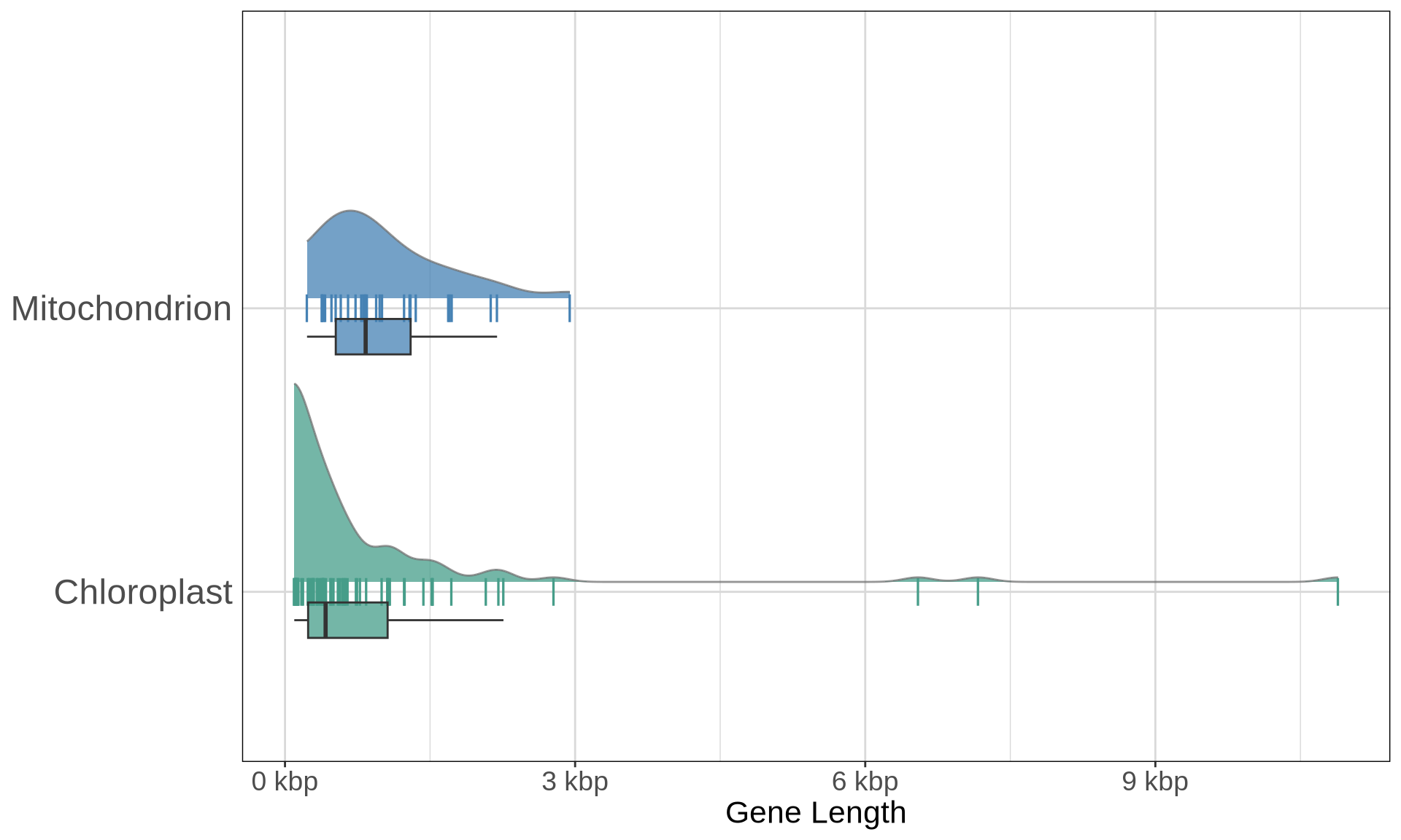

Figure 2: Alignment length distributions

On average, the mitochondrial genes seem longer than the chloroplast genes. The chloroplast genes contains 3 large outliers with the CDS alignments longer than 3 kbps, correlsponding to the three RNA polimerase genes rpoB, rpoC1, rpoC2.

1.3 Lessons Learnt

So far, we have learnt:

we have 50 Ulva isolates from 15 different Ulva species for which we have chloroplasts and mitochondrial genomes;
where the organellar genome is available, the genes present are highly conserved across Ulva isolates and species;
we have in total 99 genes (70 from the chloroplast and 29 from the mitochondria) that we can use for the downstream analyses.

1.4 Session Information

Note

R version 4.3.2 (2023-10-31)
Platform: x86_64-conda-linux-gnu (64-bit)
Running under: openSUSE Tumbleweed

Matrix products: default
BLAS/LAPACK: /home/andrea/miniforge3/envs/moai/lib/libmkl_rt.so.2;  LAPACK version 3.9.0

locale:
 [1] LC_CTYPE=en_US.UTF-8       LC_NUMERIC=C              
 [3] LC_TIME=it_IT.UTF-8        LC_COLLATE=en_US.UTF-8    
 [5] LC_MONETARY=en_US.UTF-8    LC_MESSAGES=en_US.UTF-8   
 [7] LC_PAPER=en_US.UTF-8       LC_NAME=C                 
 [9] LC_ADDRESS=C               LC_TELEPHONE=C            
[11] LC_MEASUREMENT=en_US.UTF-8 LC_IDENTIFICATION=C       

time zone: Europe/Brussels
tzcode source: system (glibc)

attached base packages:
 [1] parallel  stats4    grid      stats     graphics  grDevices utils    
 [8] datasets  methods   base     

other attached packages:
 [1] treeio_1.26.0         TreeDist_2.9.2        stringr_1.5.1        
 [4] scales_1.3.0          RColorBrewer_1.1-3    reshape_0.8.9        
 [7] phytools_2.4-4        maps_3.4.2.1          phylogram_2.1.0      
[10] phangorn_2.12.1       gridExtra_2.3         ggtree_3.10.1        
[13] ggplot2_3.5.1         ggdist_3.3.2          dplyr_1.1.4          
[16] doSNOW_1.0.20         snow_0.4-4            iterators_1.0.14     
[19] foreach_1.5.2         dendextend_1.19.0     DECIPHER_2.30.0      
[22] RSQLite_2.3.9         Biostrings_2.70.3     GenomeInfoDb_1.38.8  
[25] XVector_0.42.0        IRanges_2.36.0        S4Vectors_0.40.2     
[28] BiocGenerics_0.48.1   corrplot_0.95         ComplexHeatmap_2.18.0
[31] circlize_0.4.16       ape_5.8-1            

loaded via a namespace (and not attached):
  [1] jsonlite_1.8.9          shape_1.4.6.1           magrittr_2.0.3         
  [4] farver_2.1.2            rmarkdown_2.29          GlobalOptions_0.1.2    
  [7] fs_1.6.5                zlibbioc_1.48.2         vctrs_0.6.5            
 [10] memoise_2.0.1           RCurl_1.98-1.16         htmltools_0.5.8.1      
 [13] distributional_0.5.0    DEoptim_2.2-8           gridGraphics_0.5-1     
 [16] sass_0.4.9              bslib_0.8.0             htmlwidgets_1.6.4      
 [19] plyr_1.8.9              cachem_1.1.0            igraph_2.1.4           
 [22] mime_0.12               lifecycle_1.0.4         pkgconfig_2.0.3        
 [25] Matrix_1.6-5            R6_2.5.1                fastmap_1.2.0          
 [28] GenomeInfoDbData_1.2.11 rbibutils_2.3           shiny_1.10.0           
 [31] clue_0.3-66             digest_0.6.37           numDeriv_2016.8-1.1    
 [34] aplot_0.2.4             colorspace_2.1-1        patchwork_1.3.0        
 [37] crosstalk_1.2.1         labeling_0.4.3          clusterGeneration_1.3.8
 [40] compiler_4.3.2          bit64_4.6.0-1           withr_3.0.2            
 [43] doParallel_1.0.17       optimParallel_1.0-2     viridis_0.6.5          
 [46] DBI_1.2.3               R.utils_2.12.3          MASS_7.3-60.0.1        
 [49] rjson_0.2.23            scatterplot3d_0.3-44    tools_4.3.2            
 [52] httpuv_1.6.15           TreeTools_1.13.0        R.oo_1.27.0            
 [55] glue_1.8.0              quadprog_1.5-8          nlme_3.1-167           
 [58] R.cache_0.16.0          promises_1.3.2          reshape2_1.4.4         
 [61] cluster_2.1.8           PlotTools_0.3.1         generics_0.1.3         
 [64] gtable_0.3.6            R.methodsS3_1.8.2       tidyr_1.3.1            
 [67] pillar_1.10.1           yulab.utils_0.2.0       later_1.4.1            
 [70] lattice_0.22-6          bit_4.5.0.1             tidyselect_1.2.1       
 [73] knitr_1.49              xfun_0.50               expm_1.0-0             
 [76] matrixStats_1.5.0       DT_0.33                 stringi_1.8.4          
 [79] lazyeval_0.2.2          ggfun_0.1.8             yaml_2.3.10            
 [82] evaluate_1.0.3          codetools_0.2-20        tibble_3.2.1           
 [85] ggplotify_0.1.2         cli_3.6.3               xtable_1.8-4           
 [88] Rdpack_2.6.2            jquerylib_0.1.4         munsell_0.5.1          
 [91] Rcpp_1.0.14             coda_0.19-4.1           png_0.1-8              
 [94] blob_1.2.4              bitops_1.0-9            viridisLite_0.4.2      
 [97] tidytree_0.4.6          purrr_1.0.2             crayon_1.5.3           
[100] combinat_0.0-8          GetoptLong_1.0.5        rlang_1.1.5            
[103] fastmatch_1.1-6         mnormt_2.1.1            shinyjs_2.1.0