Chapter 2 Dimensionality Reduction and Exploration of the Merged Slides
2.1 Dimensionality Reduction
Let’s run PCA and UMAP on the merged slides to explore the data structure and relationships between the mapped voxels.
ST011 = Seurat::RunPCA(ST011, verbose = TRUE)
ST011 = Seurat::FindNeighbors(ST011, dims = 1:30)
ST011 = Seurat::FindClusters(ST011, verbose = TRUE)
ST011 = Seurat::RunUMAP(ST011, dims = 1:30)
Let’s plot the UMAP embedding of the voxels colored by the cluster assignment.
# UMAP plot
plot1 = Seurat::DimPlot(ST011, reduction = "umap", group.by = c("ident"), label = TRUE)
plot2 = Seurat::DimPlot(ST011, reduction = "umap", group.by = c("orig.ident"), cols = c("indianred", "brown2", "firebrick", "#BCD2EE", "lightskyblue3", "dodgerblue"), label = FALSE)
patchwork::wrap_plots(plot1, plot2, ncol = 2)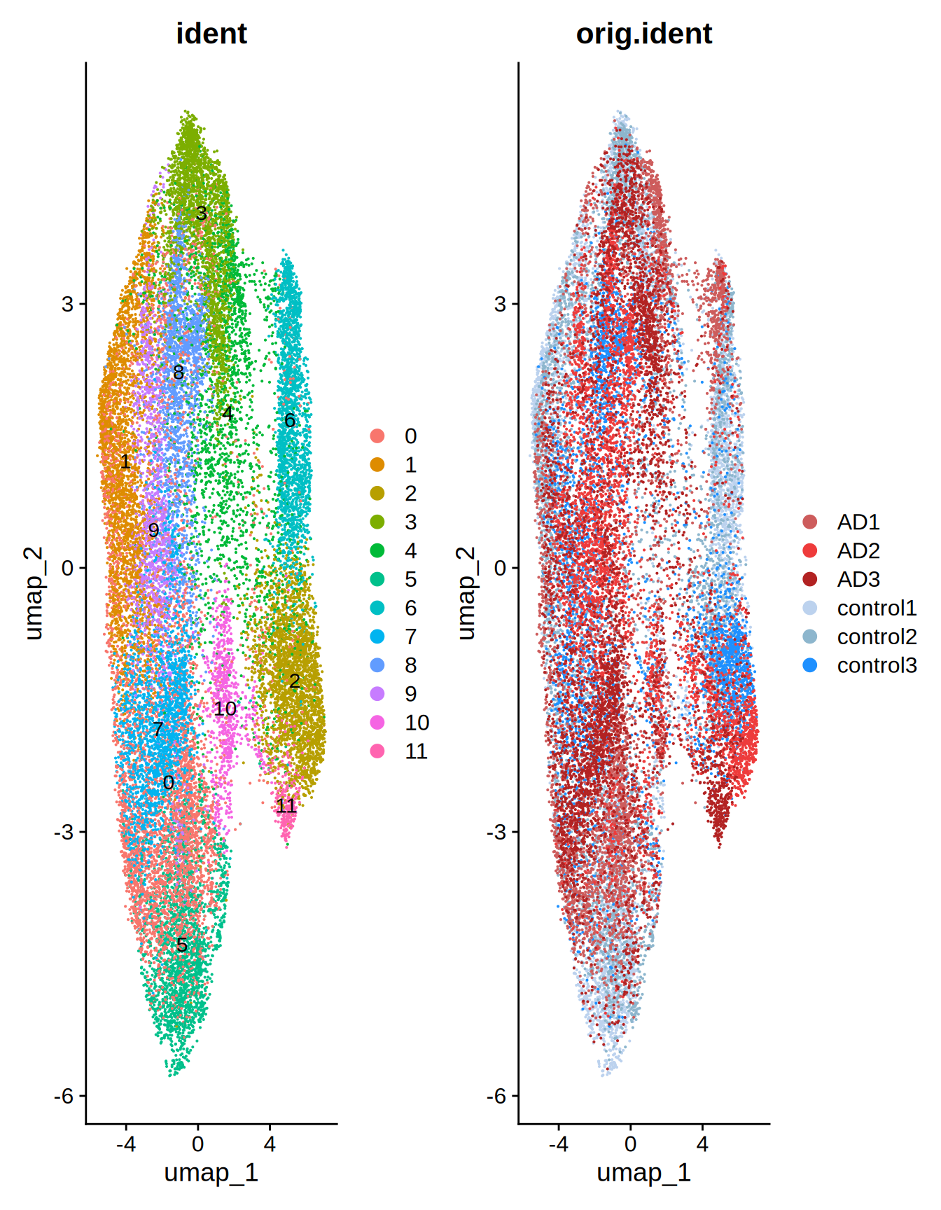
Figure 2.1: UMAP merged slides
Indeed, cell groups 9, 10 and 11 seems enriched in the AD slides. There is also an evident separation between control and AD cells in groups 2 and 5.
Let’s now overlay the Groups over the slides.
# Visualize Layers
Seurat::SpatialDimPlot(ST011, pt.size.factor = 2000, label = TRUE, label.size = 3, ncol = 3)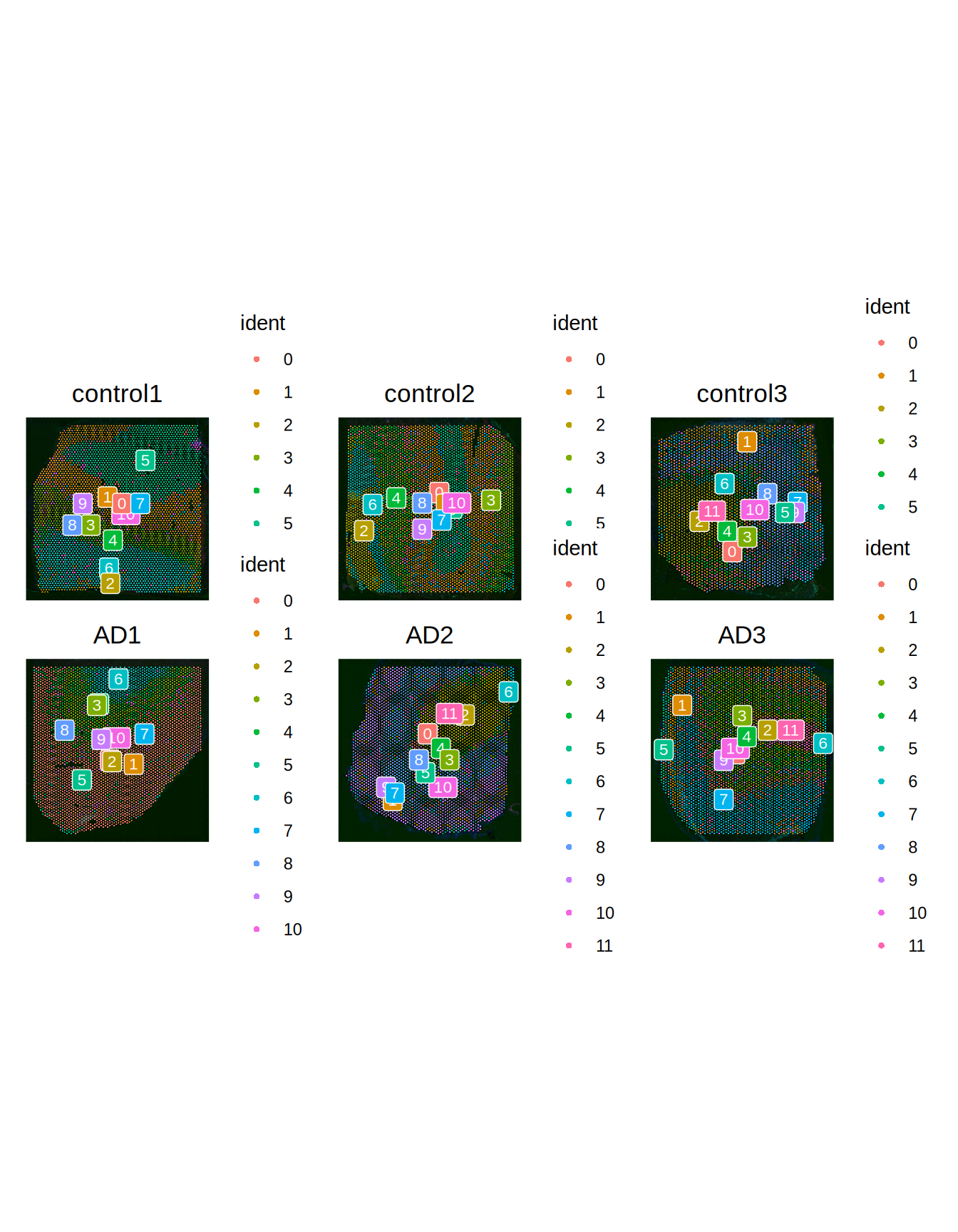
Figure 2.2: Slides VS cell groups
Let’s confirm that cell groups 9, 10 and 11 are indeed enriched in the AD slides by highlighting these cells over the slides.
# group 9
p1 = Seurat::SpatialDimPlot(ST011, images = names(ST011@images)[1],
                            cells.highlight = CellsByIdentities(object = ST011, idents = 9),
                            pt.size.factor = 2000) + NoLegend()
p2 = Seurat::SpatialDimPlot(ST011, images = names(ST011@images)[2],
                            cells.highlight = CellsByIdentities(object = ST011, idents = 9),
                            pt.size.factor = 2000) + NoLegend()
p3 = Seurat::SpatialDimPlot(ST011, images = names(ST011@images)[3],
                            cells.highlight = CellsByIdentities(object = ST011, idents = 9),
                            pt.size.factor = 2000) + NoLegend()
p4 = Seurat::SpatialDimPlot(ST011, images = names(ST011@images)[4],
                            cells.highlight = CellsByIdentities(object = ST011, idents = 9),
                            pt.size.factor = 2000) + NoLegend()
p5 = Seurat::SpatialDimPlot(ST011, images = names(ST011@images)[5],
                            cells.highlight = CellsByIdentities(object = ST011, idents = 9),
                            pt.size.factor = 2000) + NoLegend()
p6 = Seurat::SpatialDimPlot(ST011, images = names(ST011@images)[6],
                            cells.highlight = CellsByIdentities(object = ST011, idents = 9),
                            pt.size.factor = 2000) + NoLegend()
patchwork::wrap_plots(p1, p2, p3, p4, p5, p6, ncol = 3)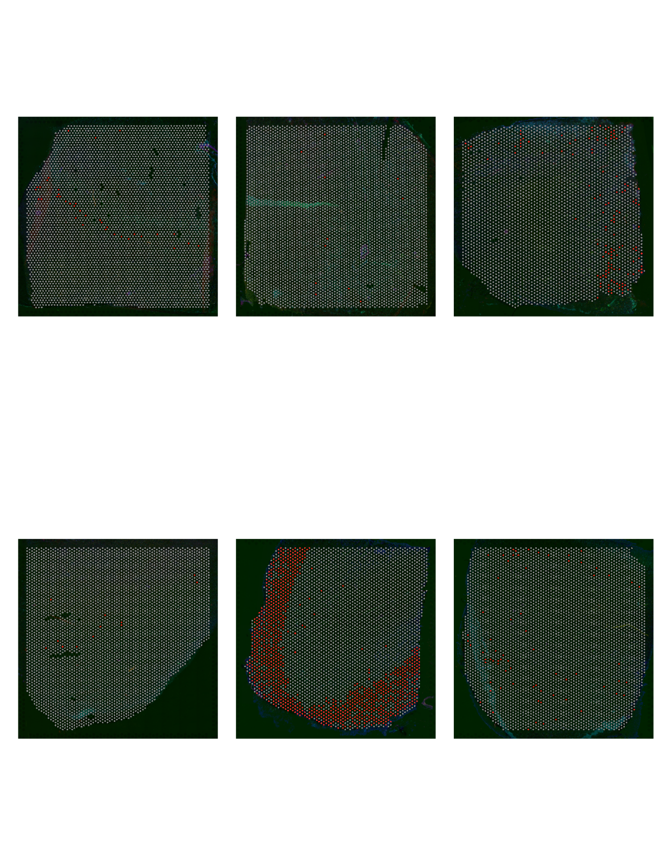
Figure 2.3: Cell Group 9 distribution
# group 10
p1 = Seurat::SpatialDimPlot(ST011, images = names(ST011@images)[1],
                            cells.highlight = CellsByIdentities(object = ST011, idents = 10),
                            pt.size.factor = 2000) + NoLegend()
p2 = Seurat::SpatialDimPlot(ST011, images = names(ST011@images)[2],
                            cells.highlight = CellsByIdentities(object = ST011, idents = 10),
                            pt.size.factor = 2000) + NoLegend()
p3 = Seurat::SpatialDimPlot(ST011, images = names(ST011@images)[3],
                            cells.highlight = CellsByIdentities(object = ST011, idents = 10),
                            pt.size.factor = 2000) + NoLegend()
p4 = Seurat::SpatialDimPlot(ST011, images = names(ST011@images)[4],
                            cells.highlight = CellsByIdentities(object = ST011, idents = 10),
                            pt.size.factor = 2000) + NoLegend()
p5 = Seurat::SpatialDimPlot(ST011, images = names(ST011@images)[5],
                            cells.highlight = CellsByIdentities(object = ST011, idents = 10),
                            pt.size.factor = 2000) + NoLegend()
p6 = Seurat::SpatialDimPlot(ST011, images = names(ST011@images)[6],
                            cells.highlight = CellsByIdentities(object = ST011, idents = 10),
                            pt.size.factor = 2000) + NoLegend()
patchwork::wrap_plots(p1, p2, p3, p4, p5, p6, ncol = 3)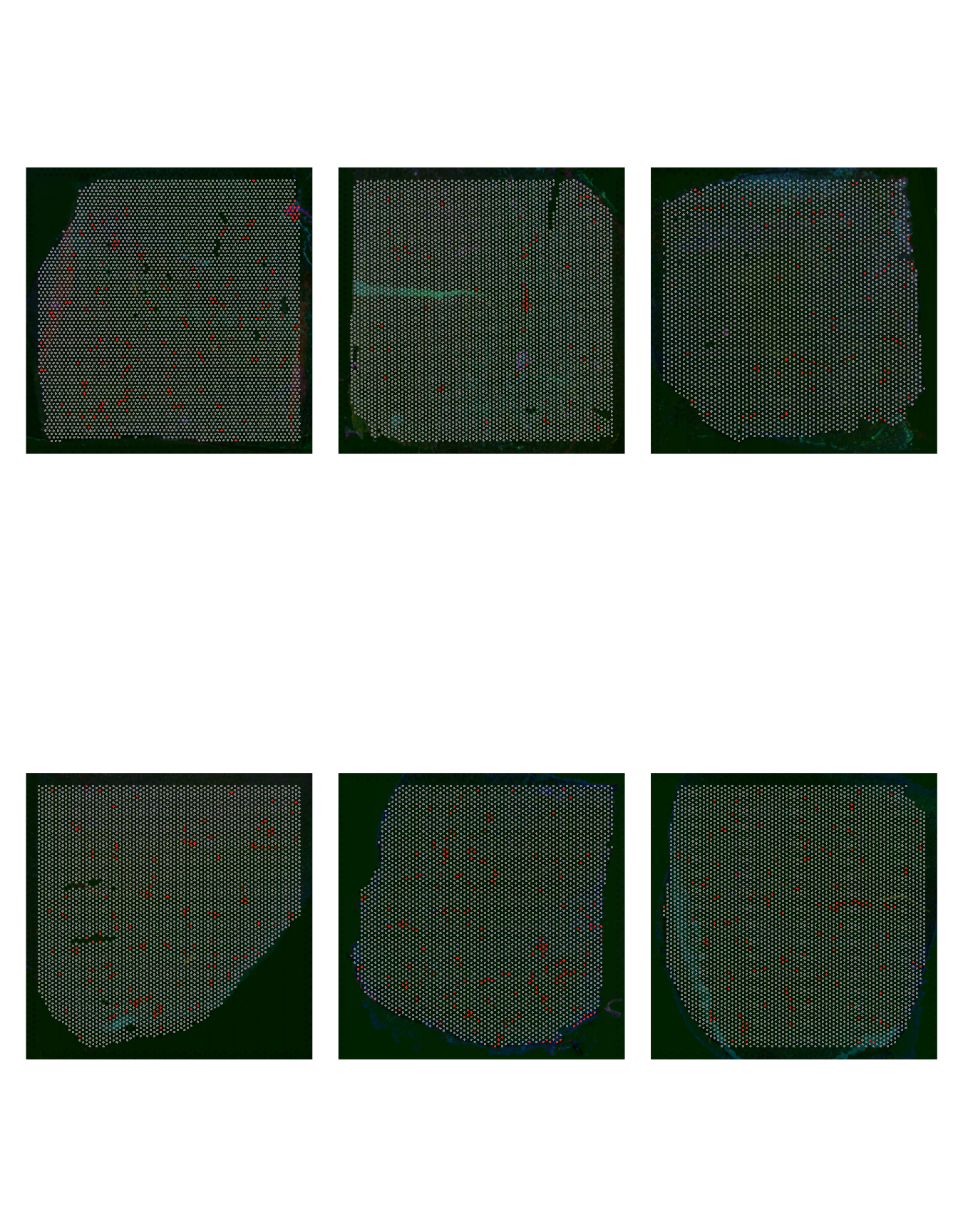
Figure 2.4: Cell Group 10 distribution
# group 11
p1 = Seurat::SpatialDimPlot(ST011, images = names(ST011@images)[1],
                            cells.highlight = CellsByIdentities(object = ST011, idents = 11),
                            pt.size.factor = 2000) + NoLegend()
p2 = Seurat::SpatialDimPlot(ST011, images = names(ST011@images)[2],
                            cells.highlight = CellsByIdentities(object = ST011, idents = 11),
                            pt.size.factor = 2000) + NoLegend()
p3 = Seurat::SpatialDimPlot(ST011, images = names(ST011@images)[3],
                            cells.highlight = CellsByIdentities(object = ST011, idents = 11),
                            pt.size.factor = 2000) + NoLegend()
p4 = Seurat::SpatialDimPlot(ST011, images = names(ST011@images)[4],
                            cells.highlight = CellsByIdentities(object = ST011, idents = 11),
                            pt.size.factor = 2000) + NoLegend()
p5 = Seurat::SpatialDimPlot(ST011, images = names(ST011@images)[5],
                            cells.highlight = CellsByIdentities(object = ST011, idents = 11),
                            pt.size.factor = 2000) + NoLegend()
p6 = Seurat::SpatialDimPlot(ST011, images = names(ST011@images)[6],
                            cells.highlight = CellsByIdentities(object = ST011, idents = 11),
                            pt.size.factor = 2000) + NoLegend()
patchwork::wrap_plots(p1, p2, p3, p4, p5, p6, ncol = 3)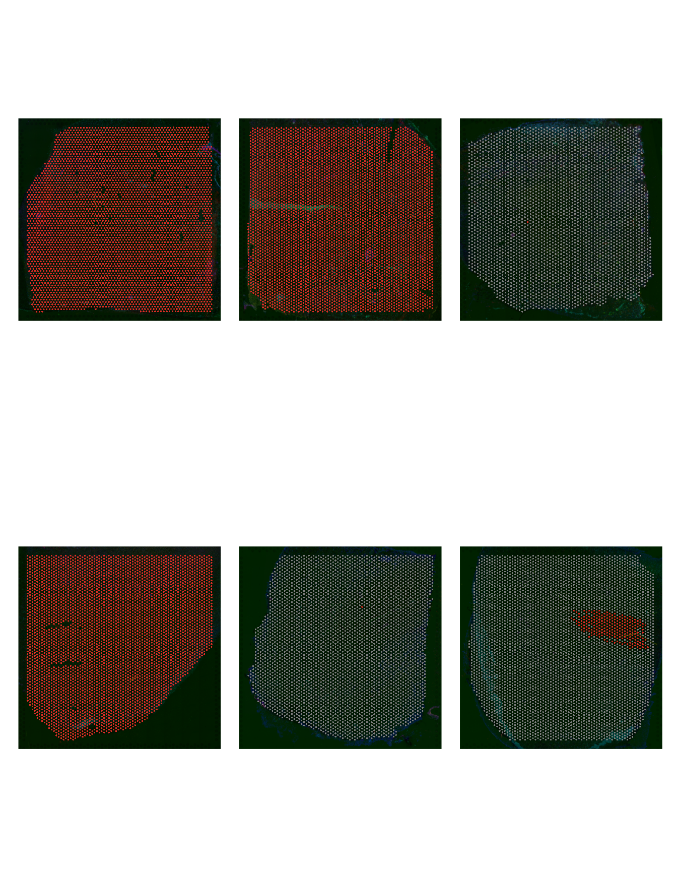
Figure 2.5: Cell Group 11 distribution
Wang et al. reports as most Differentially Expressed genes in AD vs control for these slides MTRNR2L1, MTRNR2L6, SERPINA3 and DEPP1. Let’s see the expression of these genes across the slides.
# MTRNR2L1 and MTRNR2L6 expression
Seurat::SpatialFeaturePlot(ST011, features = c("MTRNR2L1", "MTRNR2L6"), pt.size.factor = 2000)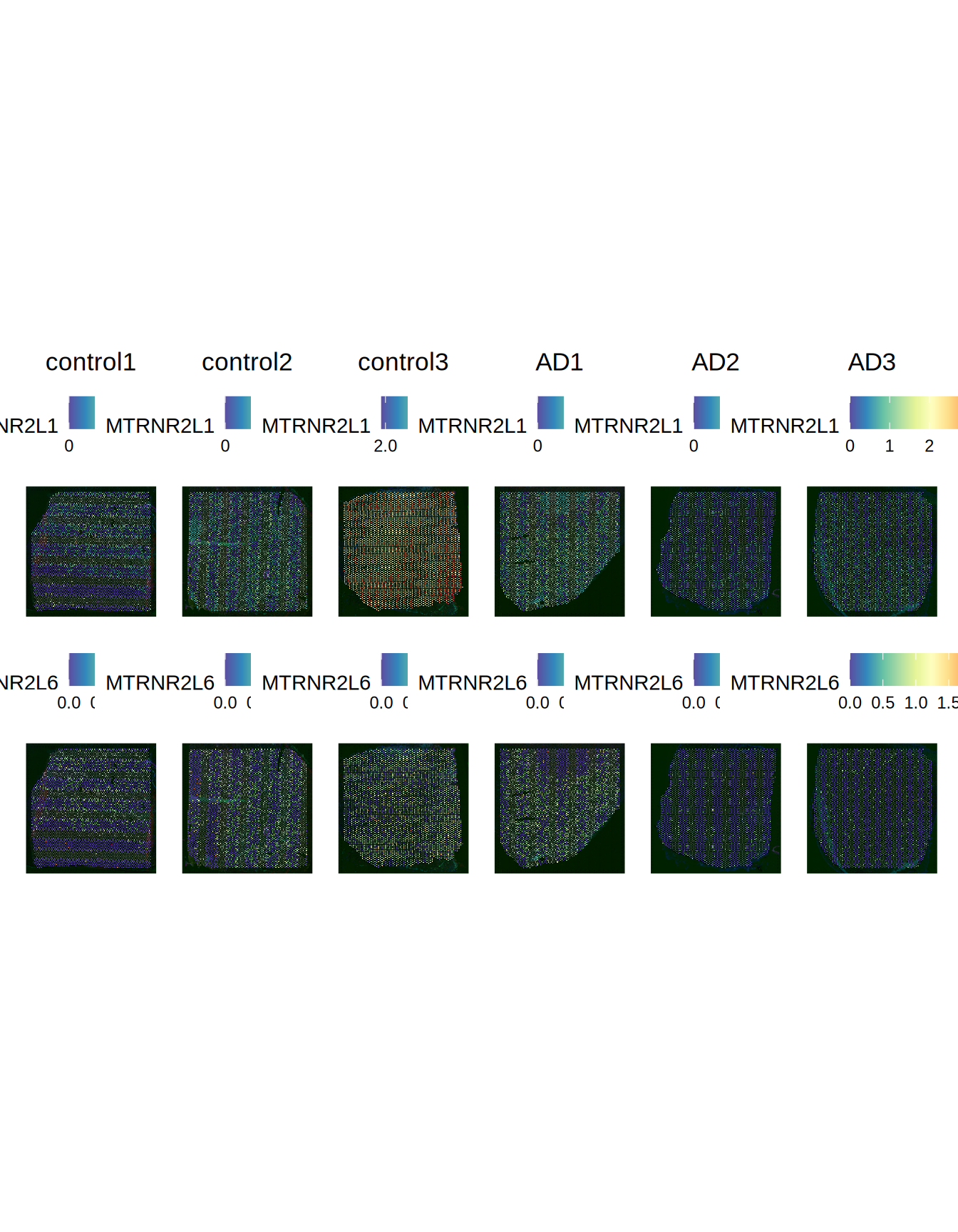
Figure 2.6: MTRNR2L1 and MTRNR2L6 expression
# DEPP1 and SERPINA3 expression
Seurat::SpatialFeaturePlot(ST011, features = c("DEPP1", "SERPINA3"), pt.size.factor = 2000)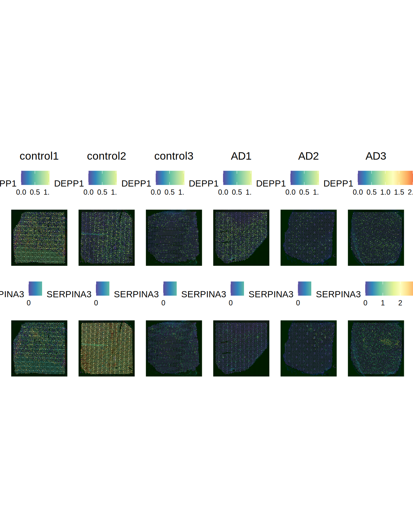
Figure 2.7: DEPP1 and SERPINA3 expression
2.2 Identification of Spatially Variable Genes across groups
We can also compute the most spatially variable genes across the slides using the FindMarkers function in Seurat.
We can choose cell groups 2 and group 11 to see which markers are more differentially expressed across these two groups.
Let’s plot the top 3 markers identified
de_markers = Seurat::FindMarkers(ST011, ident.1 = 2, ident.2 = 11)
p1 = Seurat::SpatialFeaturePlot(
    ST011,
    features = rownames(de_markers)[1:3], alpha = c(0.1, 1),
    pt.size.factor = 2000, ncol = 6
)
p1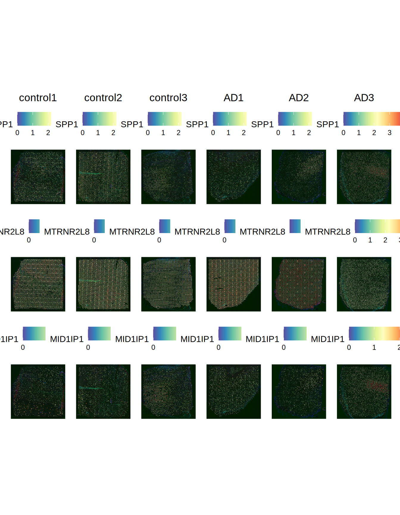
Figure 2.8: Top 3 spatially variable markers