Chapter 1 Import Slides, Exploration and Merge

1.1 Import the first Slide

The study by Chen et al. 2022 provides a dataset of spatial transcriptomics data from the human middle temporal gyrus (MTG), an area vulnerable to Alzhaimer’s Disease. The study contains six slides, 3 from AD patients and 3 from healthy controls.

The slides have been sequenced using 10X Genomics Visium technology and the raw data is available at the GEO accession number GSE220442. We have decided to retrieve the data from the ssREAD database.

We will first import one slide to explore its content.

ST01101 = qs::qread("/home/andrea/Dump/AD_spatial/ST011/ST01101.qsave")

Let’s check the content

ST01101

## An object of class Seurat 
## 36601 features across 4701 samples within 1 assay 
## Active assay: Spatial (36601 features, 2000 variable features)
##  3 layers present: counts, data, scale.data
##  2 dimensional reductions calculated: pca, umap
##  1 image present: slice1

Very well, we have an object of class Seurat containing the spatial transcriptomics data of the first slide. The object contains expression data from 36,601 genes across 4701 spots.

Let’s plot the expression of the genes next to the gene counts for each voxel in the slide.

plot1 = Seurat::VlnPlot(ST01101, features = c("nCount_Spatial")) + NoLegend()
plot2 = Seurat::SpatialFeaturePlot(ST01101, features = "nCount_Spatial", pt.size.factor = 0)
plot3 = Seurat::SpatialFeaturePlot(ST01101, features = "nCount_Spatial", pt.size.factor = 2000)
patchwork::wrap_plots(plot1, patchwork::wrap_plots(plot2, plot3, ncol = 1), ncol = 2)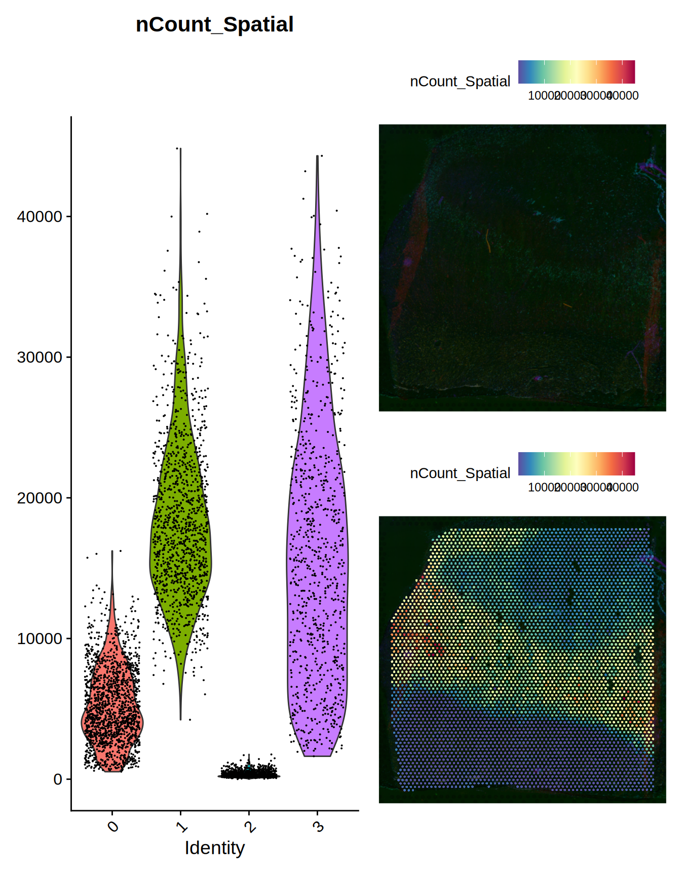

Figure 1.1: Slide ST01101 overview

1.2 Import all Slides and Merge

Now that we are familiar with the content of the first slide, let’s import them in batch and merge them into a single Seurat object.

First, we import the slides into the list ST011_list. Each slide is also transfermed using the Seurat::SCTransform function. Since the images attached to each sample have all the same name, we also make sure that we change the orig.ident of each slide so that the images are not overwritten when we merge the slides together.

slides_names = data.frame(
    slide = c("ST01101", "ST01102", "ST01103", "ST01104", "ST01105", "ST01106"),
    slide_name = c("control1", "control2", "control3", "AD1", "AD2", "AD3")
)

# load slides data
ST011_list = list()
for(k in 1:6){

    # get name
    slide_name = slides_names$slide[k]
    slide_type = slides_names$slide_name[k]

    ST011_list[[slide_type]] = qs::qread(paste0("/home/andrea/Dump/AD_spatial/ST011/ST0110", k, ".qsave"))
    ST011_list[[slide_type]]$orig.ident = slide_type

    # expression normalization
    ST011_list[[slide_type]] = Seurat::SCTransform(ST011_list[[slide_type]], assay = "Spatial", verbose = TRUE)

    gc()

}

Then, we merge the slides into a single Seurat object ST011 and set the variable features to the union of the variable features of the individual slides.

# merge
ST011 = merge(x = ST011_list[[1]], y = ST011_list[2:length(ST011_list)])
Seurat::VariableFeatures(ST011) = c(
    Seurat::VariableFeatures(ST011_list[[1]]),
    Seurat::VariableFeatures(ST011_list[[2]]),
    Seurat::VariableFeatures(ST011_list[[3]]),
    Seurat::VariableFeatures(ST011_list[[4]]),
    Seurat::VariableFeatures(ST011_list[[5]]),
    Seurat::VariableFeatures(ST011_list[[6]])
)
names(ST011@images) = slides_names$slide_name
gc()

ST011

## An object of class Seurat 
## 59009 features across 25293 samples within 2 assays 
## Active assay: SCT (22408 features, 18000 variable features)
##  3 layers present: counts, data, scale.data
##  1 other assay present: Spatial
##  2 dimensional reductions calculated: pca, umap
##  6 images present: control1, control2, control3, AD1, AD2, AD3

We can now plot the expression across clusters splitted by slide.

# expression QC
Seurat::VlnPlot(ST011, features = c("nCount_Spatial"), split.by = "orig.ident") +
    scale_fill_manual(values = c("indianred", "brown2", "firebrick",
                                 "#BCD2EE", "lightskyblue3", "dodgerblue")) +
    ggplot2::theme(legend.position = c(0.9, 0.9))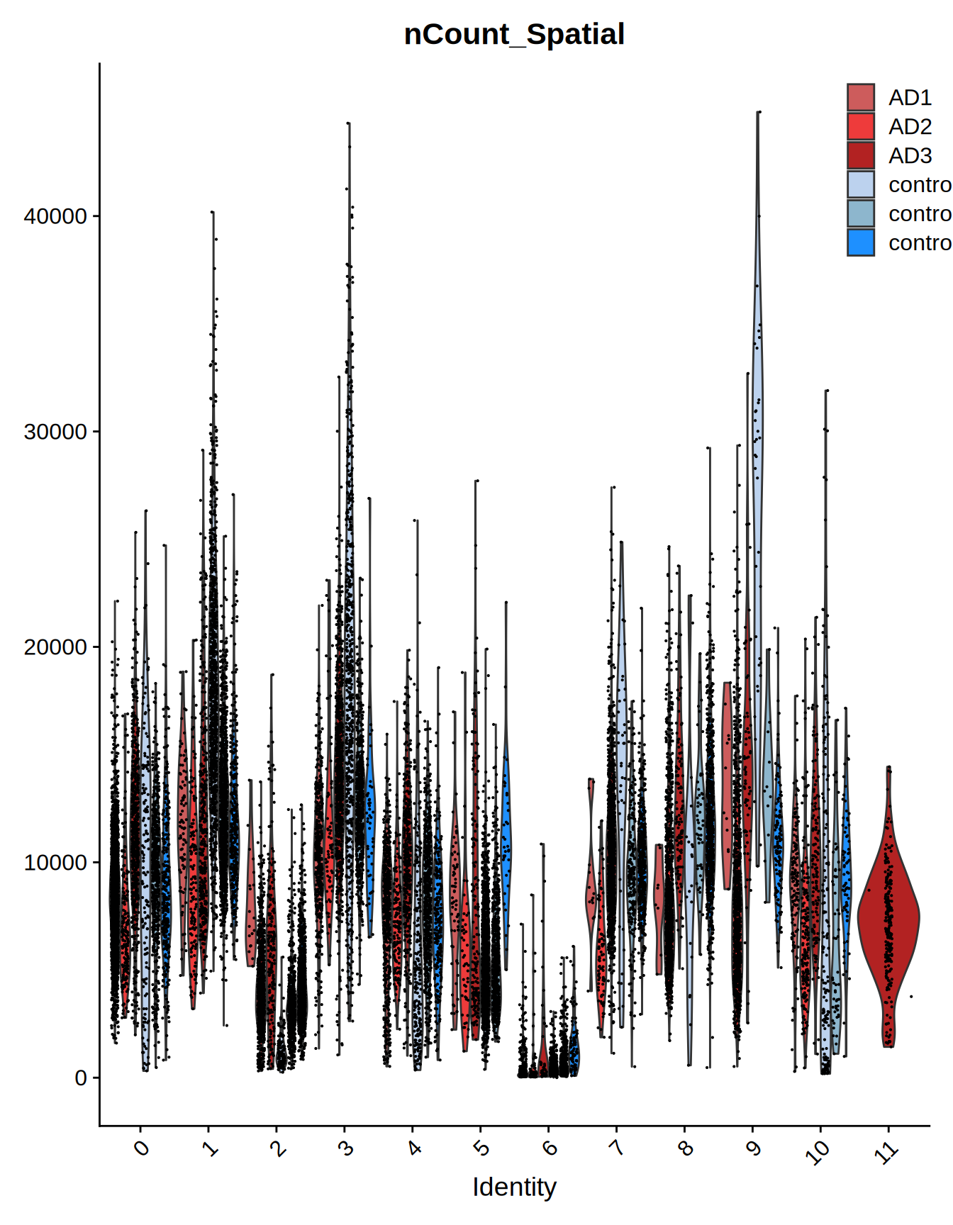

Figure 1.2: Merged slides overview - Violin Plot

We can immediatly notice how the control group have an higher cell counts and expression values for group 2 and 5, while the AD slides seems encriched in cells from group 9. Group 11 appear only in an AD slide.

Let’s check as well how the gene counts are distributed across the six slides.

# expression QC
plot1 = Seurat::SpatialFeaturePlot(ST011, features = "nCount_Spatial", pt.size.factor = 0)
plot2 = Seurat::SpatialFeaturePlot(ST011, features = "nCount_Spatial", pt.size.factor = 2000)
patchwork::wrap_plots(plot1, plot2, ncol = 1)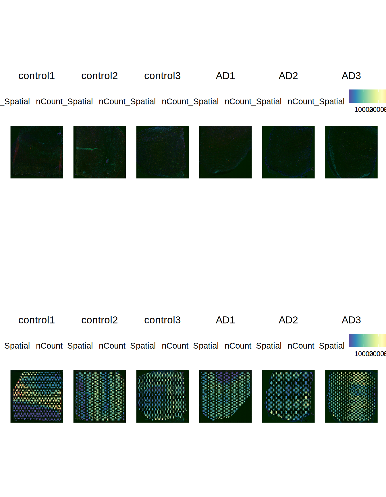

Figure 1.3: Merged slides overview - Slides expression

Now we have a single Seurat object ST011 containing all the slides. We can proceed with the Dimensionality Reduction steps.