Chapter 3 Load and Prepare the Allen GTM Atlas

The full Allen Brain Cell Atlas is an incredible resource, but it is so large that it is very challenging to use it on a laptop. I have tried to download and downsapled it to just 10% of the amount of cells it contains. I had to reserve ~300Gb of my harddrive as extra swap not to run out of RAM. In the end, the process was so cumbersome, that I had to recline to a more manageable asset. Well, to be fair the Atlas comes as an anndata file, and while istalling the right libraries in python I broke my hd5f libraries in R, so I could not transform anndata to Seurat after downsampling, and so I have looked for a Seurat-compatible colution :/.

I have retrieve the MTG reference from the Allen Brain Cell Atlas from the Seattle Alzheimer’s Disease Brain Cell Atlas (SEA-AD). The Seurat object provided is much more maneageable (~4.4 Gb) and it contains targeted information to annotate our slides.

Let’s import the Atlas.

# import
allen_MTG_reference = qs::qread("/home/andrea/Dump/AD_spatial/allen_MTG_reference.qsave", nthreads = 4)

Let’s check the Atlas content.

allen_MTG_reference

## An object of class Seurat 
## 59236 features across 888263 samples within 1 assay 
## Active assay: RNA (59236 features, 0 variable features)
##  1 layer present: data
##  2 dimensional reductions calculated: UMAP, tSNE

We run some dimensionality reduction on it, since the UMAP is available but not the PCA.

# it comes without PCA, so we run it
allen_MTG_reference = Seurat::FindVariableFeatures(allen_MTG_reference, selection.method = "vst", nfeatures = 2000)
allen_MTG_reference = Seurat::ScaleData(allen_MTG_reference)
allen_MTG_reference = Seurat::RunPCA(allen_MTG_reference, verbose = TRUE)
allen_MTG_reference = Seurat::FindNeighbors(allen_MTG_reference, dims = 1:30)
allen_MTG_reference = Seurat::FindClusters(allen_MTG_reference, verbose = TRUE)

The clustering process identifies 127 communities, of them 90 are flagged as singletons resulting in 37 final cell clusters. We can also plot number of cells per Region of Interest and for each cell type.

# visualize Atlas frequencies breakdown
p1 = ggplot(as.data.frame(t(table(allen_MTG_reference$ROIGroupFine))), aes(x = Var2, y = Freq)) +
    geom_bar(aes(fill = Var2), color = "grey35", stat = "identity") +
    geom_text(aes(label = Freq), size = 8, hjust = 1.1) +
    scale_fill_manual(values = c(brewer.pal(8, "Set2"), brewer.pal(8, "Dark2"))) +
    scale_y_log10(breaks = scales::trans_breaks("log10", function(x) 10^x),
                  labels = scales::trans_format("log10", scales::math_format(10^.x))) +
    labs(title = "Region", y = "Number of cells") +
    coord_flip() +
    theme(plot.title = element_text(size = 24, hjust = 0.5),
          axis.title.x = element_text(size = 18),
          axis.title.y = element_blank(),
          axis.text = element_text(size = 14),
          panel.background = element_rect(fill = NA, colour = "black"),
          panel.grid.major.x = element_line(colour = "grey"),
          panel.grid.major.y = element_blank(),
          legend.position = "none")

p2 = ggplot(as.data.frame(t(table(allen_MTG_reference$cell_type))), aes(x = Var2, y = Freq)) +
    geom_bar(aes(fill = Var2), color = "grey35", stat = "identity") +
    geom_text(aes(label = Freq), size = 8, hjust = 1.1) +
    scale_fill_manual(values = c(brewer.pal(11, "Set3"))) +
    scale_y_log10(breaks = scales::trans_breaks("log10", function(x) 10^x),
                  labels = scales::trans_format("log10", scales::math_format(10^.x))) +
    labs(title = "Cell type", y = "Number of cells") +
    coord_flip() +
    theme(plot.title = element_text(size = 24, hjust = 0.5),
          axis.title.x = element_text(size = 18),
          axis.title.y = element_blank(),
          axis.text = element_text(size = 14),
          panel.background = element_rect(fill = NA, colour = "black"),
          panel.grid.major.x = element_line(colour = "grey"),
          panel.grid.major.y = element_blank(),
          legend.position = "none")

patchwork::wrap_plots(p1, p2, ncol = 1)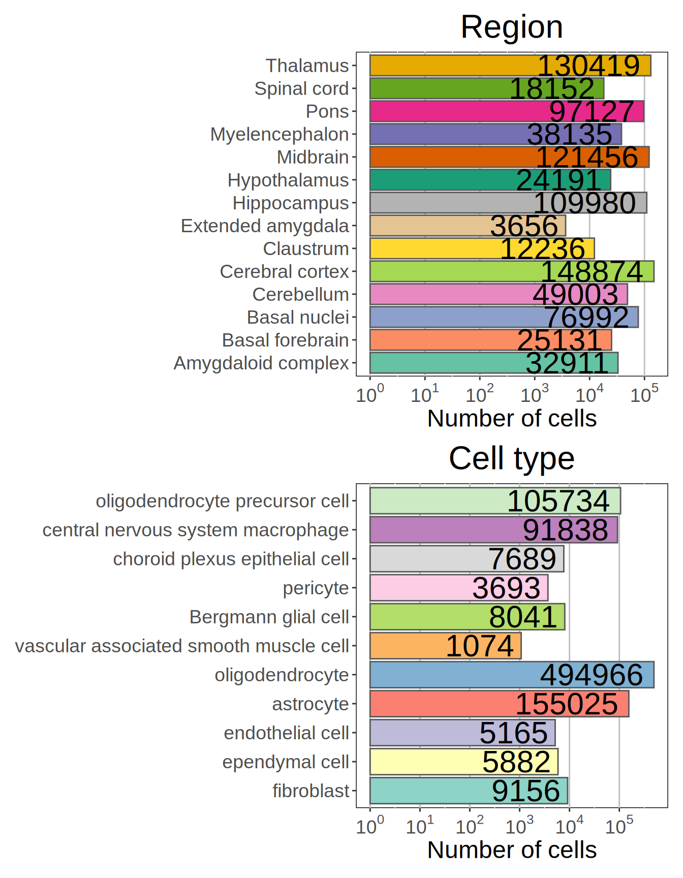

Figure 3.1: Number of cells per Region of Interest

Let’s see how these regions and cell types are distributed in the UMAP space.

# Visualize UMAPs of region and cell type of the Atlas
p1 = Seurat::DimPlot(allen_MTG_reference, group.by = "ROIGroupFine", label = FALSE, raster = FALSE) +
    scale_color_manual(values = c(brewer.pal(8, "Set2"), brewer.pal(8, "Dark2")))
p2 = Seurat::DimPlot(allen_MTG_reference, group.by = "cell_type", label = FALSE, raster = FALSE) +
    scale_color_manual(values = c(brewer.pal(11, "Set3")))
patchwork::wrap_plots(p1, p2, ncol = 1)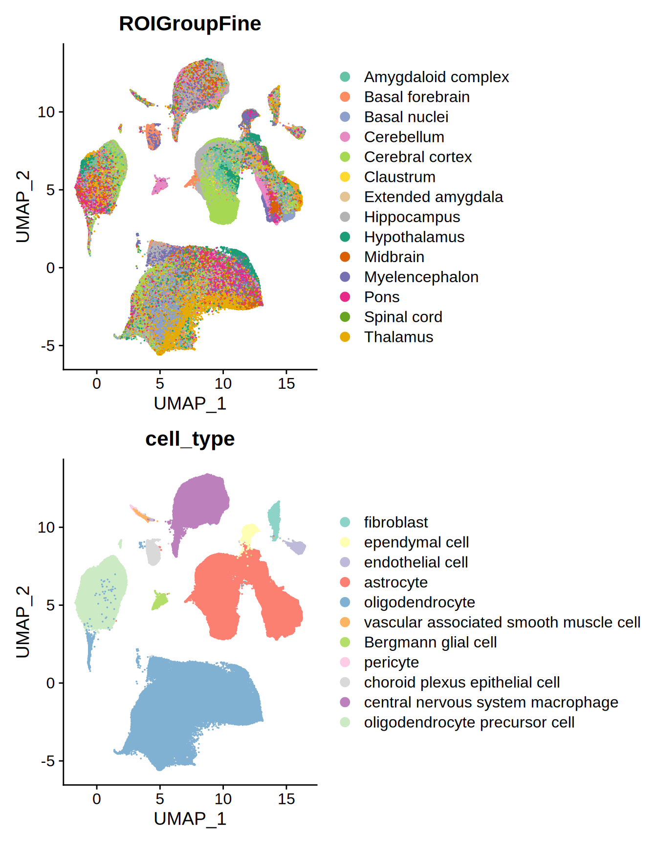

Figure 3.2: UMAP Allen MTG reference

In the next chapter we will use the Allen MTG reference to annotate our slides and perform a spatial deconvolution to estimate the cell type composition of the Visium spots.