Gather Datasets and QC

Gather resources

We can gather cancer multi-omics datasets from large public data resources such as TCGA (The Cancer Genome Atlas) and the GDC (Genomic Data Commons), as well as smaller-scale datasets generated by individual labs from the USDC Xena platform. From the Xena platform, we can find the data from Pan-Cancer Atlas consortium, which provides textbook high quality datasets that can be explored for target discovery in cancer.

TCGA PanCan collects 12,839 samples from 28 organs, 69 primary sites spanning 32 different cancer types.

The metadata available for the samples and the subjects include:

biopsys type (metastatic, primary tumor, solid tissue normal) –> data
cancer subtype based on canonical molecular classification (methylation, miRNA, mRNA, proteins, etc.) –> data
cancer subtype based on the immune models –> data
overall survival information –> data

For these samples, there are available rich clinical metadata and matched multiomics datasets.

We can retrieved the following multiomics readouts:

copy number variants at the gene level –> data
DNA methylation data –> data
gene expression (RNAseq) –> data
micro RNAs (miRNA) –> data
protein expression –> data
somatic mutations –> data

All the multiomics readouts are at the gene level, except for the DNA methylation data, that will have to be mapped and normalized at the gene level. Luckily, a mapping file is available as well.

Xena provides as well already precomputed enrichments and cell types deconvolutions:

gene programs that are canonical drug targets –> data
homologous recombination deficiency (HRD) –> data
immune signaling –> data
ssGSEA PARADIGM annotations –> data
stemness score based on DNA methylation signals –> data
stemnsess score based on the RNAseq expression of 103 key genes –> data

I assure you that integrating all these data will be fun, and it will provide deep insights on each cancer we decided to analyse.

Samples Overview

Next step is to integrate together all the available sample and subjects metadata. This allows to break down the samples by cancer type and demographic distributions. While Xena provides some information, it lacks a cleaned table containing all the demographic information of the subjects. Conveniently, GitHub user ipezoa already retrieved from GDC and CGC and combined together all the metadata obtained from JSON and XML files. A thorough explanation of each metadata field is reported here.

Let’s integrate all the metadata together. We have indeed access to a rich and comprehensive ensemble of clinical and sample metadata for the samples at hand.

Cohort demographics

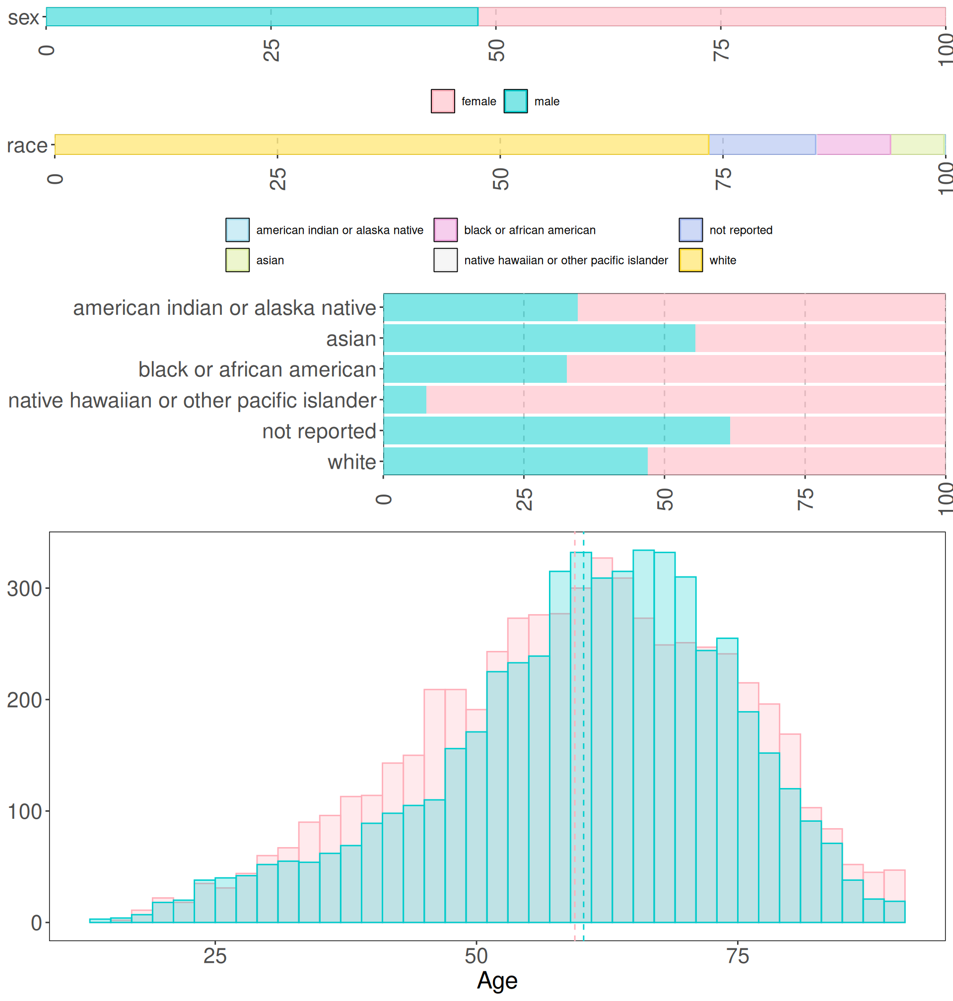
Let’s check the overall demographic distributions of all the samples.

We notice that the ration between males and females included in the PanCan dataset is almost 1:1. As well, the age distributions for both sexes are very similar, and the averages of the two distributions almost overlap around 60 years old (59.4 years for female and 60.3 years for males). Race-wise, we have an over-representation of whites (73,4% of samples), followed by 12.0% of samples for which no race information is available. Blacks or african americans and asian represent a small percentage of the samples available, with 8.3% and 6.0% of the samples respectively.

Clinical overview

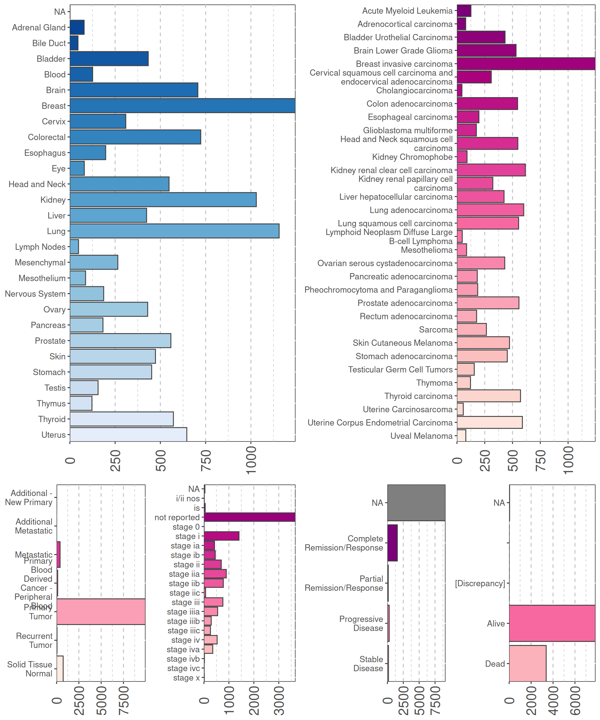
Let’s check now the different cancer included in the study.

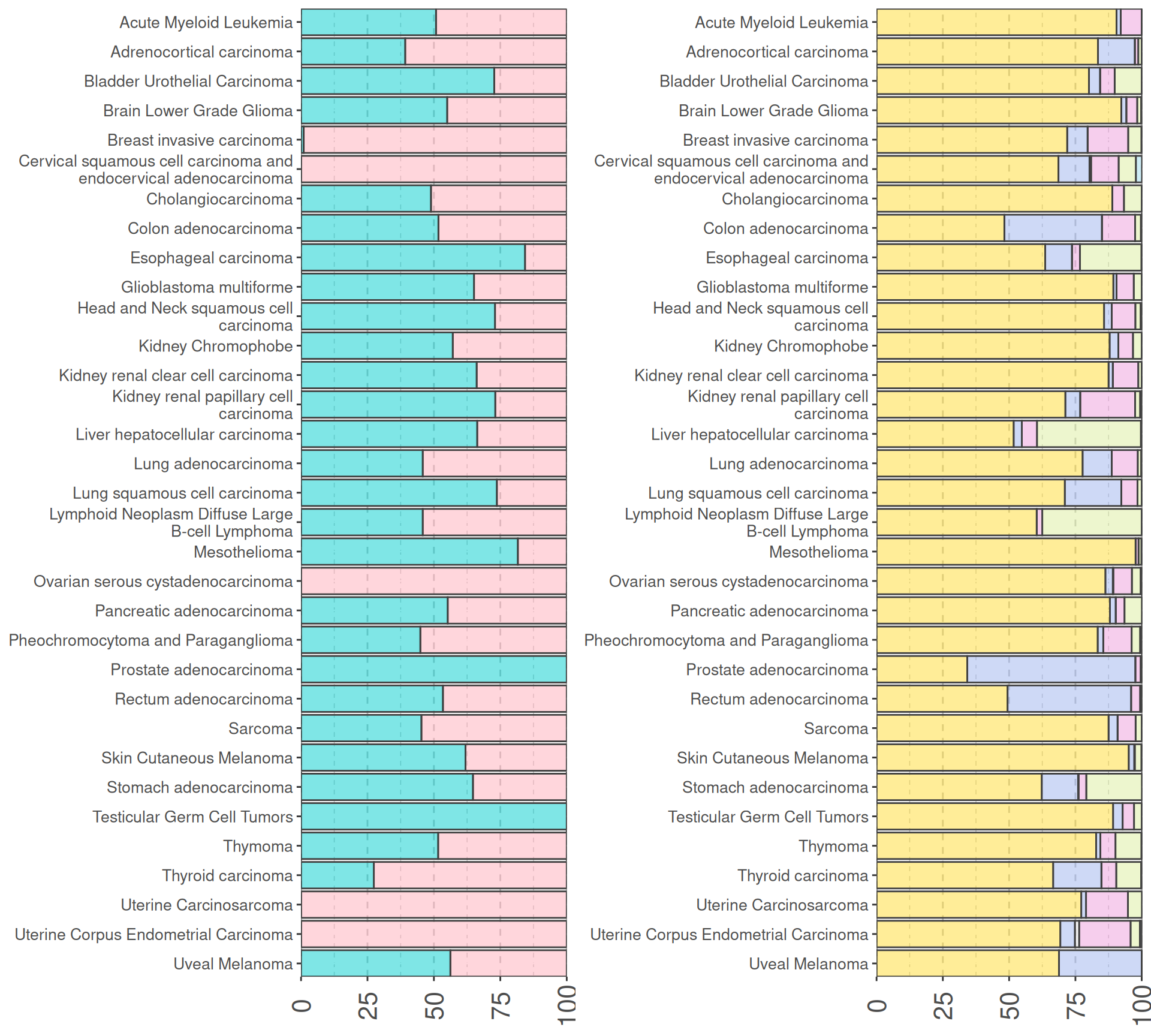
We can check for any biases in terms of sex and ethnicity in the collected cancer samples. I would not expect any surprise here. Let’s see.

Figure 3: Clinical metadata breakdown by sex and ethnicity.

To have a first overview of all the samples, we will plot a UMAP based on the gene expression of all the biopsys. A UMAP is an algorithm for dimension reduction based on manifold learning techniques and ideas from topological data analysis. The UMAP algorithm first constructs a weighted graph of the data in input (with N-dimensions), where the weight in the graph edge corresponds to how similar is a point (i.e.: sample) to the next one, and then projects this similarity graph into a bi-dimensional space. The 2-D projection is optimized to faithfully represents the relationships between the points in the N-dimensional space.

To build the UMAP, we focus on the 1,000 top most variable genes between the transcriptomics samples. This allows us to maximize similarities and differences between sample groups (if any).

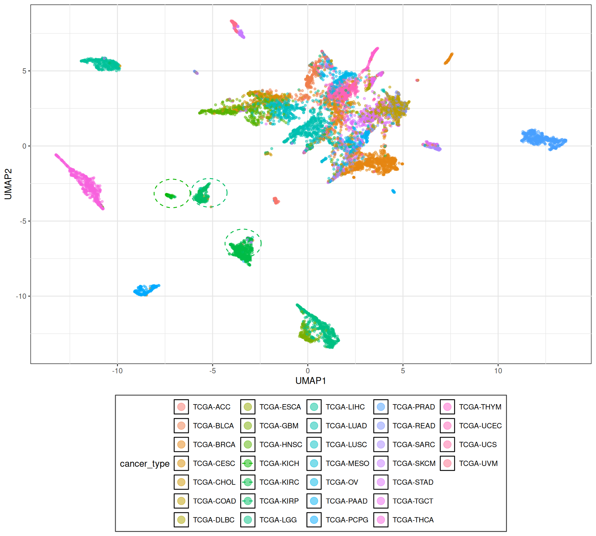
The UMAP show us that we can clearly clusters cancer types in distinct groups, and that we can identify clusters with related cancers (i.e.: colon-adenocarcinoma COAD and rectum-adenocarcinoma READ).

Among the sample clusters generated by the UMAP, we can identify three distinct cluters in the center of the UMAP (highlighted by dotted circles) that loosely correspond to the three kidney cancer subtypes in this cohort: kidney chromophobe (KICH), kidney renal papillary cell carcinoma (KIRP), and kidney renal clear cell carcinoma (KIRC).

Lessons Learnt

So far, we have learnt:

TCGA is a public resource with a wide collection of samples from cancer biopsies from patients affected by 32 different cancer types.
TCGA provides abundant molecular and clinical information for both biopsies and patients and it allows for patient stratification and therapeutic target discovery.
Cancers with kidneys as primary sites are the third most abundant samples available in TCGA (n = 1,030 samples), after breast (n = 1,246) and lung biopsies (n = 1,156), and provides an excellent yet challenging case-study.

Session Information

Note

R version 4.3.3 (2024-02-29)
Platform: x86_64-pc-linux-gnu (64-bit)
Running under: Ubuntu 24.04.3 LTS

Matrix products: default
BLAS:   /usr/lib/x86_64-linux-gnu/blas/libblas.so.3.12.0 
LAPACK: /usr/lib/x86_64-linux-gnu/lapack/liblapack.so.3.12.0

locale:
 [1] LC_CTYPE=en_US.UTF-8    LC_NUMERIC=C            LC_TIME=C              
 [4] LC_COLLATE=en_US.UTF-8  LC_MONETARY=C           LC_MESSAGES=en_US.UTF-8
 [7] LC_PAPER=C              LC_NAME=C               LC_ADDRESS=C           
[10] LC_TELEPHONE=C          LC_MEASUREMENT=C        LC_IDENTIFICATION=C    

time zone: Europe/Brussels
tzcode source: system (glibc)

attached base packages:
[1] grid      stats     graphics  grDevices utils     datasets  methods  
[8] base     

other attached packages:
 [1] umap_0.2.10.0      stringr_1.5.1      scales_1.4.0       RColorBrewer_1.1-3
 [5] matrixStats_1.5.0  gridExtra_2.3      ggplot2_3.5.2      forcats_1.0.0     
 [9] edgeR_4.0.16       limma_3.58.1       DT_0.33            dplyr_1.1.4       
[13] data.table_1.17.8  cowplot_1.2.0     

loaded via a namespace (and not attached):
 [1] sass_0.4.10       generics_0.1.4    stringi_1.8.7     lattice_0.22-5   
 [5] digest_0.6.37     magrittr_2.0.3    evaluate_1.0.4    fastmap_1.2.0    
 [9] jsonlite_2.0.0    Matrix_1.6-5      RSpectra_0.16-2   crosstalk_1.2.1  
[13] jquerylib_0.1.4   cli_3.6.5         rlang_1.1.6       cachem_1.1.0     
[17] withr_3.0.2       yaml_2.3.10       tools_4.3.3       locfit_1.5-9.12  
[21] reticulate_1.43.0 vctrs_0.6.5       R6_2.6.1          png_0.1-8        
[25] lifecycle_1.0.4   htmlwidgets_1.6.4 pkgconfig_2.0.3   pillar_1.11.0    
[29] bslib_0.9.0       gtable_0.3.6      glue_1.8.0        Rcpp_1.1.0       
[33] statmod_1.5.0     xfun_0.52         tibble_3.3.0      tidyselect_1.2.1 
[37] knitr_1.50        dichromat_2.0-0.1 farver_2.1.2      htmltools_0.5.8.1
[41] labeling_0.4.3    rmarkdown_2.29    compiler_4.3.3    askpass_1.2.1    
[45] openssl_2.3.3

On this page