2 Transcriptomics Analysis

2.1 On this page

Biological insights and take-home messages are at the bottom of the page at Lesson Learnt: Section 2.6.

Here we investigate the transcriptomics data across the three Kidney Cancers.
First we filter lowly expressed genes and we do some exploratory analyses on samples, gene expression and clinical covariates.
We then run a formal Differential Gene Expression analysis to identify genes that have different expression levels across the three Kidney cancer types.
We perform Gene Set Enrichment Analyses on the differentially expressed genes to investigate biological and molecular themes that discriminates between the three Kidney cancer types.
Finally, we characterize the tumour micro-environments of the three Kidney cancer types by quantifying the tumour-infiltrating immune cells.

2.2 Filtering of lowly abundant genes

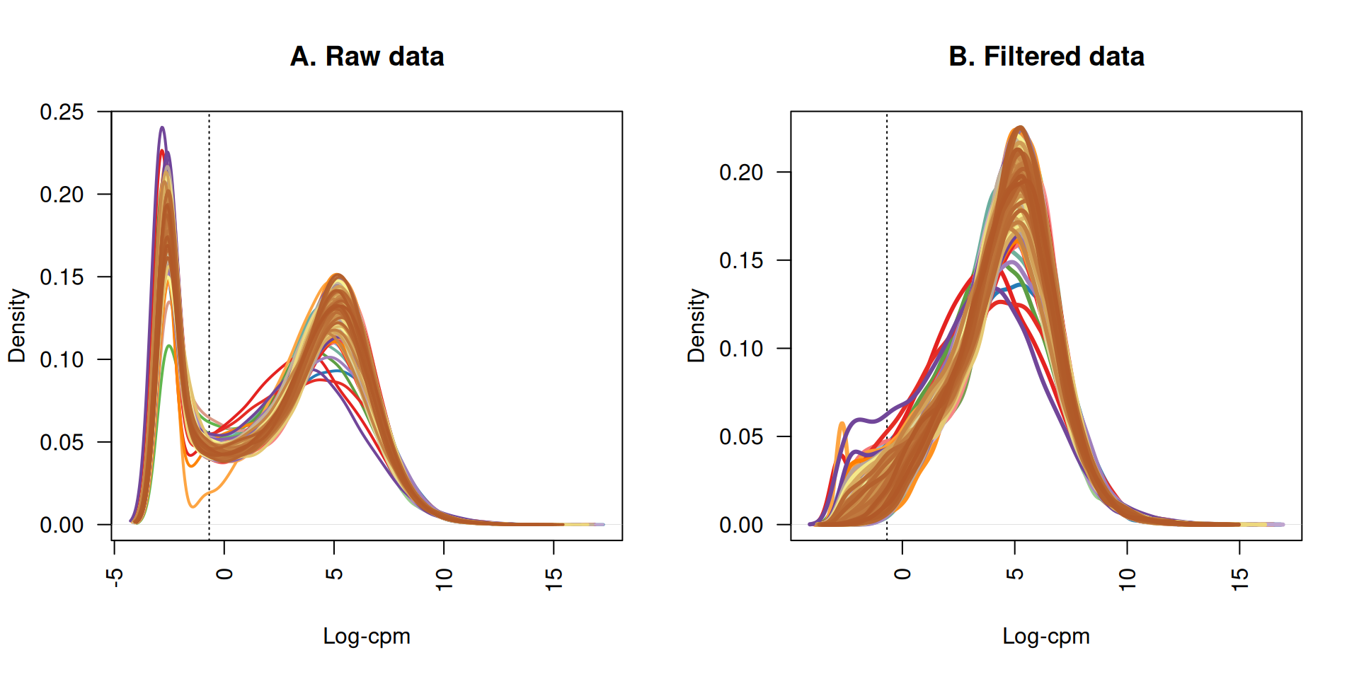
The first step for transcriptomics analysis is to filter genes that are lowly expressed across all samples because they just inflate the data matrix and they do not contribute to the detection of the biological signal.

The filtering step results in the removal of 6,472 genes. The graph below reports the density curves of gene expressions (logCPM) before and after filtering of lowly expressed genes. Each line represent a sample. Before filtering, all samples showed a left-hand side shoulder, with a peak below 0 logCPM higher than a second peak centered around 5 logCPM. The peak below 0 logCPM represent all the lowly to non-expressed genes. After filtering, only expressed genes are retained.

Figure 1: Filtering Lowly Expressed Genes.

2.3 Dimesionality Reduction and Dataset Exploration

2.3.1 Principal Component Analysis (PCA)

The Principal Component Analysis (PCA) is an unsupervised linear dimensionality reduction technique that summarizes large amount of information (as the one in a transcriptomics count table) into a smaller set of summarized variables (Principal Components) that capture the linear relationships between the data. In a transcriptomics dataset, the number of Principal Components equals the number of samples.

The PCA algorithm is run in an iterative manner: the first Principal Component is calculated by finding the line that maximizes the variance between the samples. The second Principal Component is calculated in the same way, with the condition that it is uncorrelated with (i.e., perpendicular to) the first principal component and that it accounts for the next highest variance. The third Principal Component is calculated in the same way, down to the last Principal Component.

To run PCA analyses on transcriptomics data, I recommend the PCAtools package by Kevin Blighe and Aaron Lun.

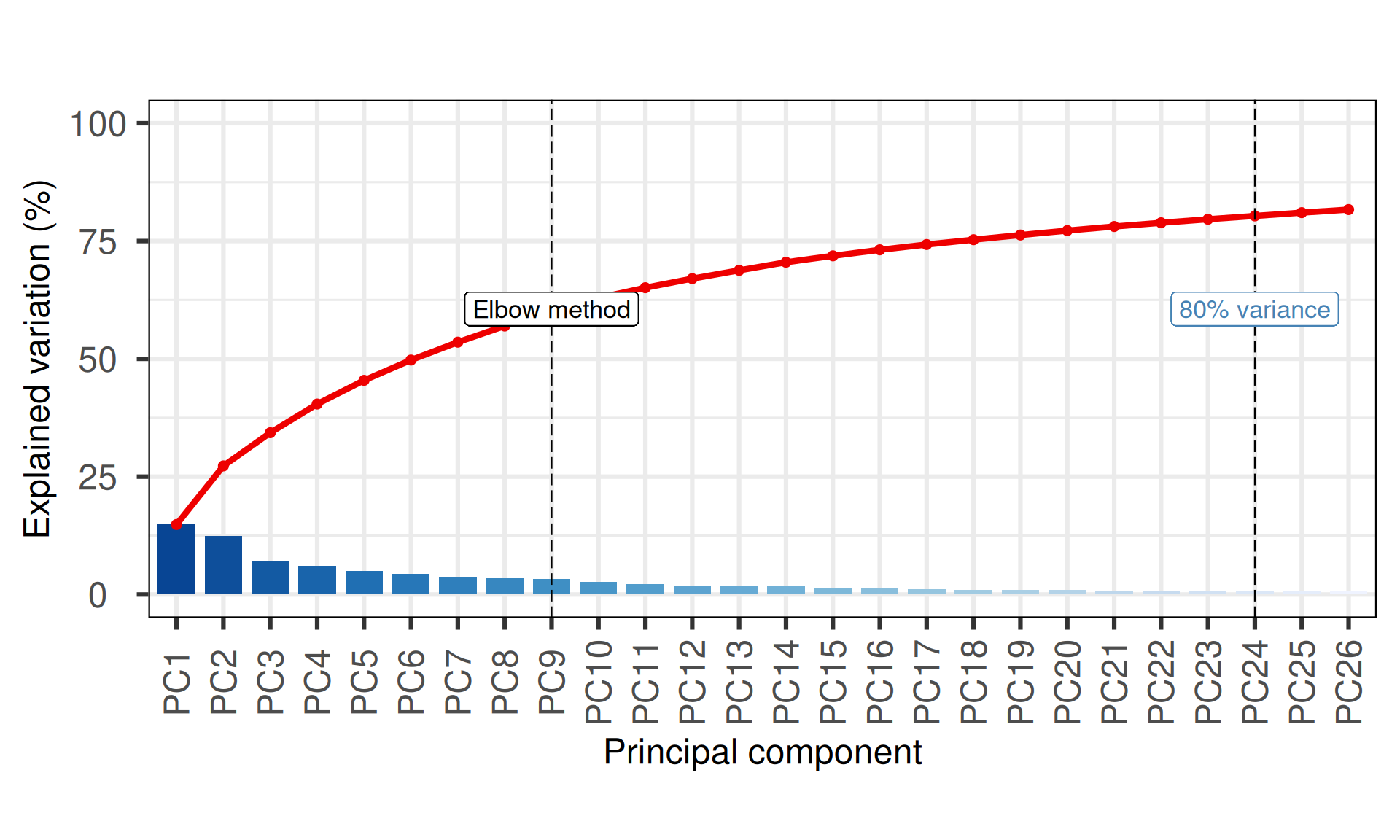
The first 24 Principal Components capture more than 80% of the variance in the Kidney cancers transcriptomics dataset, with the first two components (PC1 and PC2) capturing a bit more than 25% of the variance.

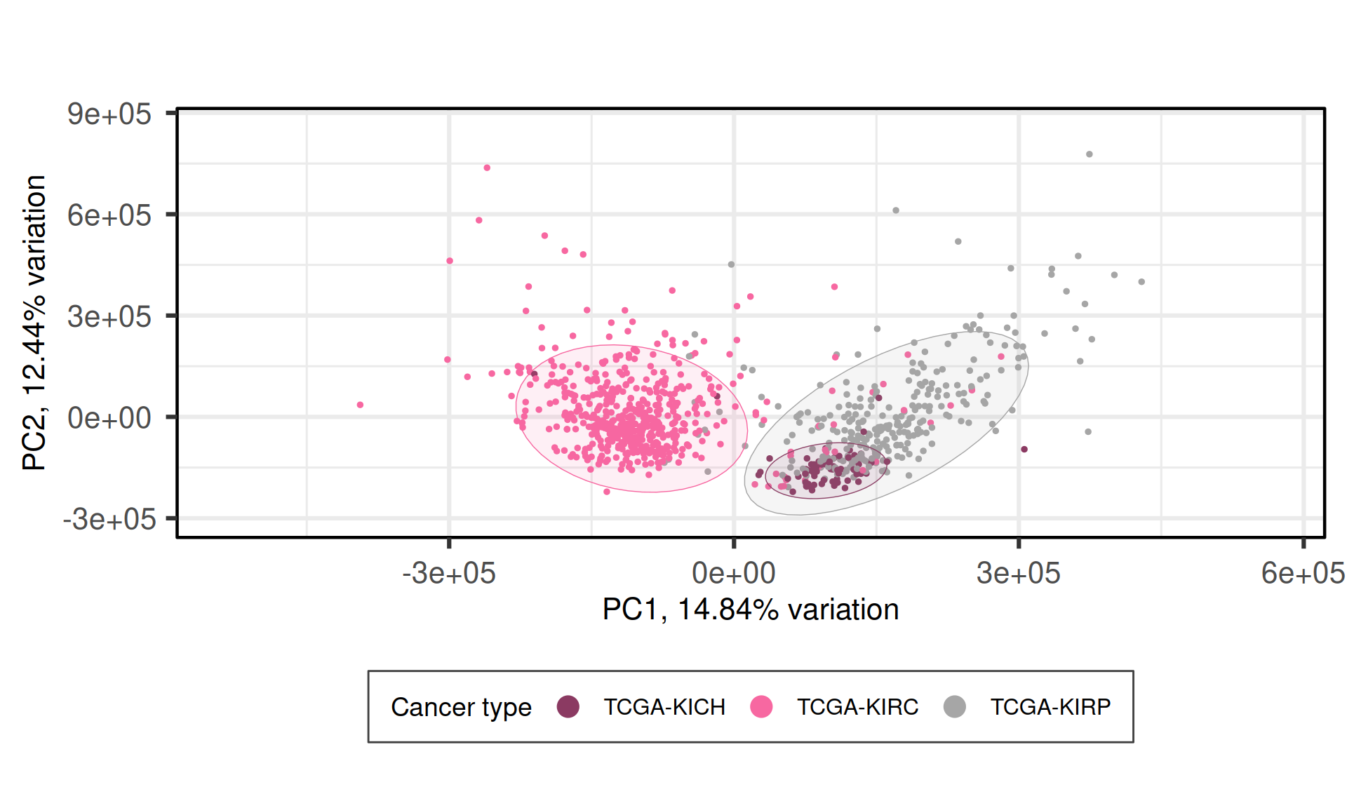
When we project the samples in the PC1 and PC2, we can see that the PC1 separates KIRC from KICH adn KIRP, which instead cluster together. The second component PC2, instead, seems to partially separate KICH and KIRP samples.

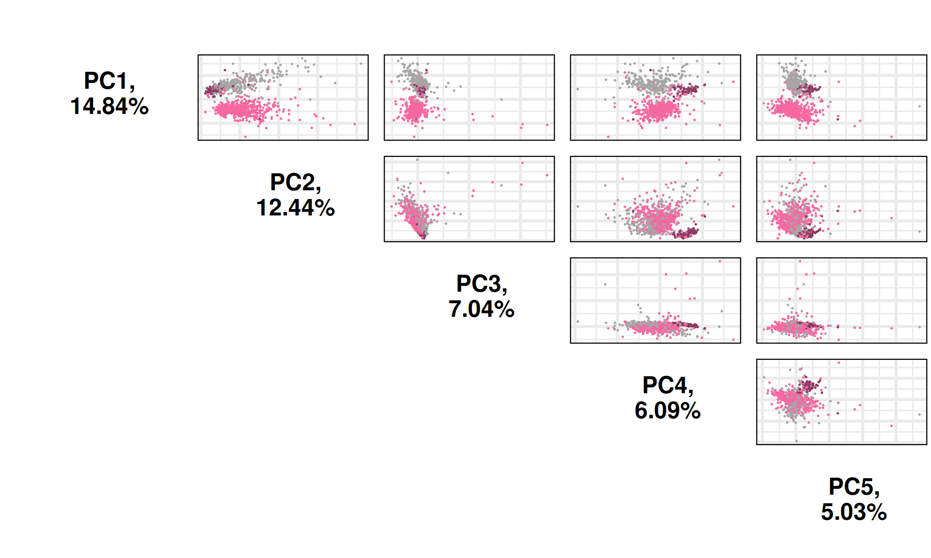
We can also investigate other dimensions Principal Components, to see if there is a component that manages to fully resove the three cancer types. PC4 seems to separates better the KICH from KIRP, while PC1 can discriminate between KIRC and KIRP.

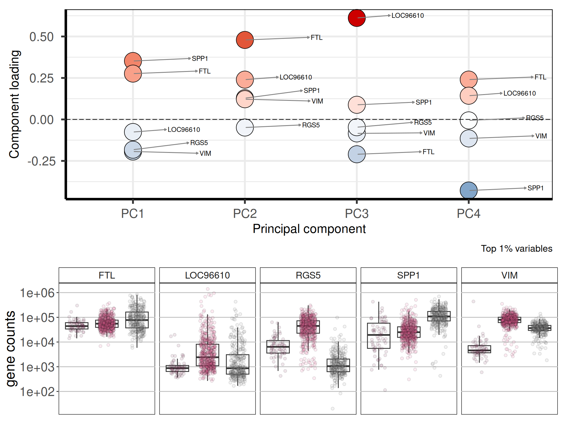
Let’s check the loadings (i.e.: 24 Principal Components capture more than 80% of the variance in the) for the top 4 Principal Components. These indicate which genes are the more responsible to explain the position of the samples along the components, and the direction of this separation.

Looking at the top 1% most variable genes (~ 140 genes), the following 5 genes are the top loadings for the first 4 Principal Components:

Let’s now check the expression of the five top genes identified with the PCA across the cancer types:

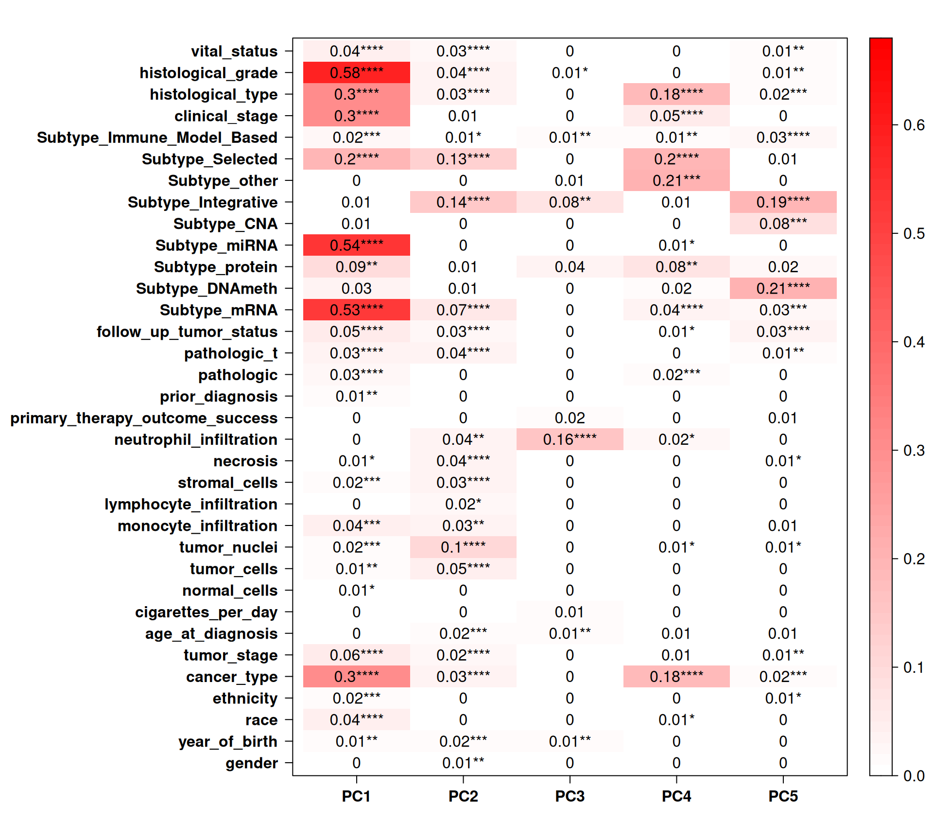
Let’s check the Pearson correlation with other clinical covariates.

Certain histological and molecular subtyping correlates perfectly with PC4 (which discriminates KICH) immune infiltrating cells also correlates with PC1 and PC2, and may help to further characterize the subtypes and stratify patients

As we have learnt before (Chapter 1), KIRC patients seems to had a worse outcome than KIRP and to have tumors in more advanced stages. PC1 (computed from transcriptomics data) clearly separates KIRC and KIRP samples, and it correlates with tumor histological grade and stage, as well as clinical outcome. This show that we have good correlation between clinical observations and gene expression in Kidney cancers.

Sadly, no correlation between the top 5 components and the outcome of therapeutic care.

Figure 6: PCA, correlations between clinical covariates and Principal Components.

2.4 Differential gene expression analysis

Differential gene expression (DGE) analysis is used compare gene expression levels between two or more sample groups, in this case, Kidney cancer types. DGE can help in identifying genes involved in a particular biological process, providing information on gene regulation and underlying biological mechanisms. One of the most used approaches to identify associations between genes and biological consist in applying generalized linear models, which aims to assign the variation in gene expression to each known variable in the experimental design, such as patient age, ethnicity, cancer type, treatment center taking care of the patients, etc.

In the section above we saw that age, ethnicity (and race) and age had somewhat a correlation with the cancer types. Therefore, we include this covariates in the differential gene expression analysis in order to take their contribution to gene expression variance into account.

Now, we will compare the gene expression across the three different Kidney cancer types, and we will test the following pairwise comparisons for genes that are differentially expressed: KICH vs KIRC, KICH vs KIRP and KIRC vs KIRP.

2.4.1 Identification of differentially expressed genes

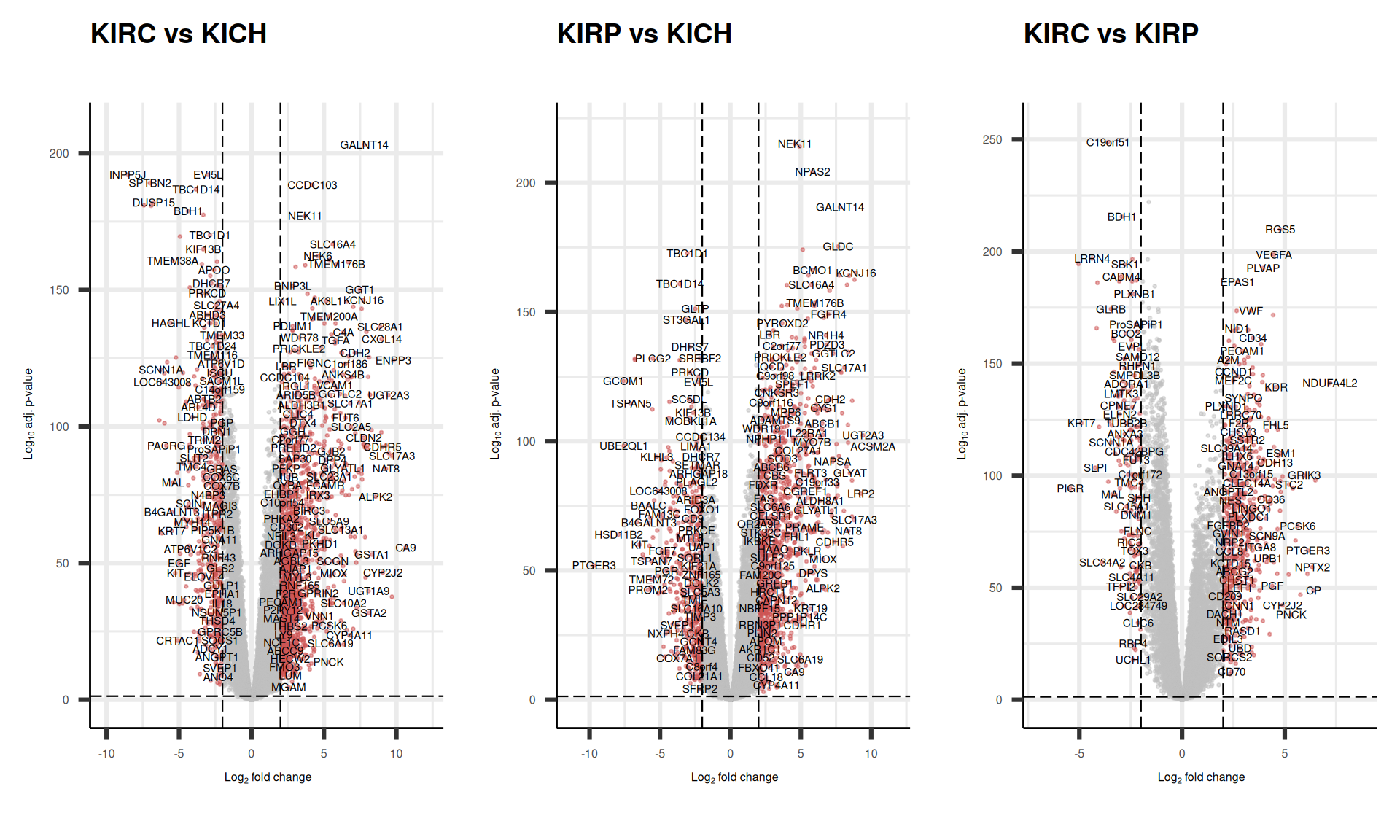
For transcriptomics analyses, we use two arbitrary thresholds to retain genes that are significantly differentially expressed across the each comparison: an absolute logFold-Change (logFC) higher than 2, and an adjusted p-value lower than 0.05. This results in:

KIRC_vs_KICH, 2,058 differentially expressed genes, 1,553 upregulated and 505 downregulated
KIRP_vs_KICH, 1,567 differentially expressed genes, 1,101 upregulated and 466 downregulated
KIRC_vs_KIRP, 739 differentially expressed genes, 570 upregulated and 169 downregulated

The relationships between how much a gene is differentially expressed (logFC) and its likelihood to be observed (p-value) in a DGE comparison is often visualized with a volcano plot, where each dot represent a gene. There are hundreds of genes that are differentially expressed across the biopsies of the three different kidney cancers in our cohorts.

Figure 7: Volcano plots of each contrats reporting the genes differentially expressed.

We can also check the logFC and adjusted p-value for the top 5 genes that are the top loadings for the first 4 Principal Components and see how these genes were differentially expressed across the comparisons. We can confirm what we have naively observed at the level of gene counts in Figure 6 while investigating the PCA loadings: while these 5 genes have been suggested has the top loadings of the 2 Principal Components, FTL seems to do not have a large difference in expression across the three Kidney tumours.

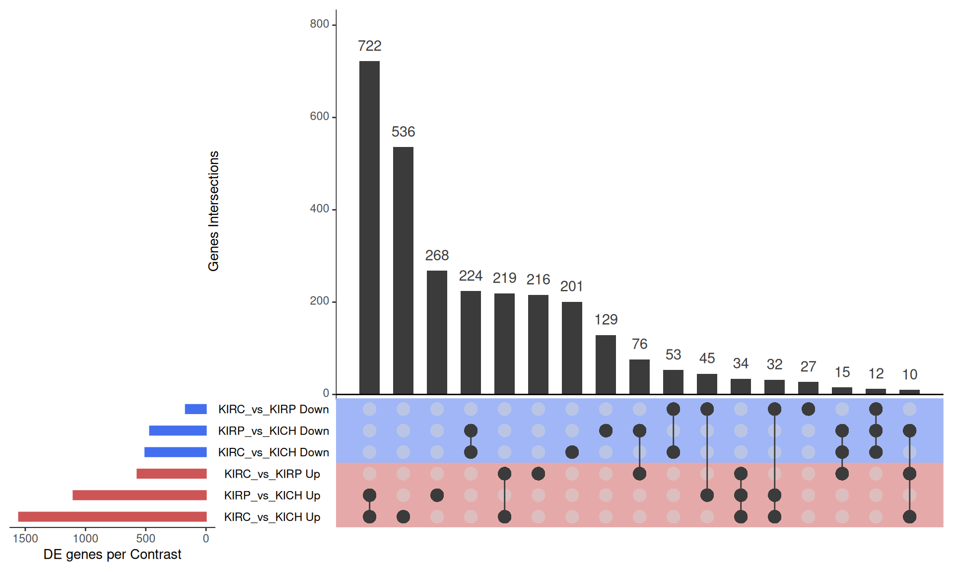
We can further dig into the hundreds of genes that are differentially expressed by looking at the overlaps between the upregulated and downregulated genes across the three DGE comparisons. The UpSet plot below facilitates visualizing these overlaps. As seen in the PCA, PC1 explain ~15% of the variability observed in the genes, and it separates KIRC from KICH and KIRP kidney cancer. We would then expect a large overlap between KIRC_vs_KIRP and KIRC_vs_KICH DE genes, however, we see instead that the largest overlaps between DE genes are between KIRC_vs_KICH and KIRP_vs_KICH comparisons. This suggest that KIRC and KIRP are more similar to each other than KICH, suggesting a more complex relationship than the one observed in the first two principal components.

Figure 8: UpSet reporting the genes differentially expressed upregulated and downregulated in common across all contrasts.

Tables of differentially expressed genes.

2.4.2 Comparative enrichment analyses across cancer types

In the next steps we further characterized the hundreds of genes that are differentially expressed across the three kidney cancers by performing a Gene Set Enrichment Analysis (GSEA). GSEA can identify whether specific pathways or molecular functions are upregulated or downregulated across the entire list of genes, providing insight into the biological differences at the gene expression levels between the three kidney cancers.

We will perform GSEA against an annotated set of gene ontologies and pathways:

Gene Ontology (GO). Gene Ontology provides a a comprehensive, computational model of biological systems and it is the world’s largest source of information on the functions of genes. It provides terms organized in three hierarchical ontologies (BP, CC and MF), that provide insights over gene Biological Processes (BP), Cellular Compartments (CC) and Molecular Functions (MF).
Kyoto Encyclopedia of Genes and Genomes pathways (KEGG). KEGG is a database resource for understanding high-level functions and utilities of the biological system, such as the cell, the organism and the ecosystem, from molecular-level information. KEGG pathway is a collection of manually drawn pathway maps representing our knowledge of the molecular interaction, reaction and relation networks.
Reactome Pathways. Reactome is a free, open-source, curated and peer-reviewed pathway database.
WikiPathways. WikiPathways is an open science platform for biological pathways contributed, updated, and used by the research community.

2.4.2.1 GO Biological Process terms

Gene Ontology Biological Process are the larger processes or ‘biological programs’ accomplished by the concerted action of multiple molecular activities. Examples of broad BP terms are “DNA repair” or “signal transduction”. Examples of more specific terms are “cytosine biosynthetic process” or “D-glucose transmembrane transport”.

Figure 9: dotplot of enriched GO Biological Process terms.

Figure 10: Term maps reporting relationships between GO Biological Process across the different contrasts.

Figure 11: gene maps reporting relationships between GO Biological Process enriched across the different contrasts

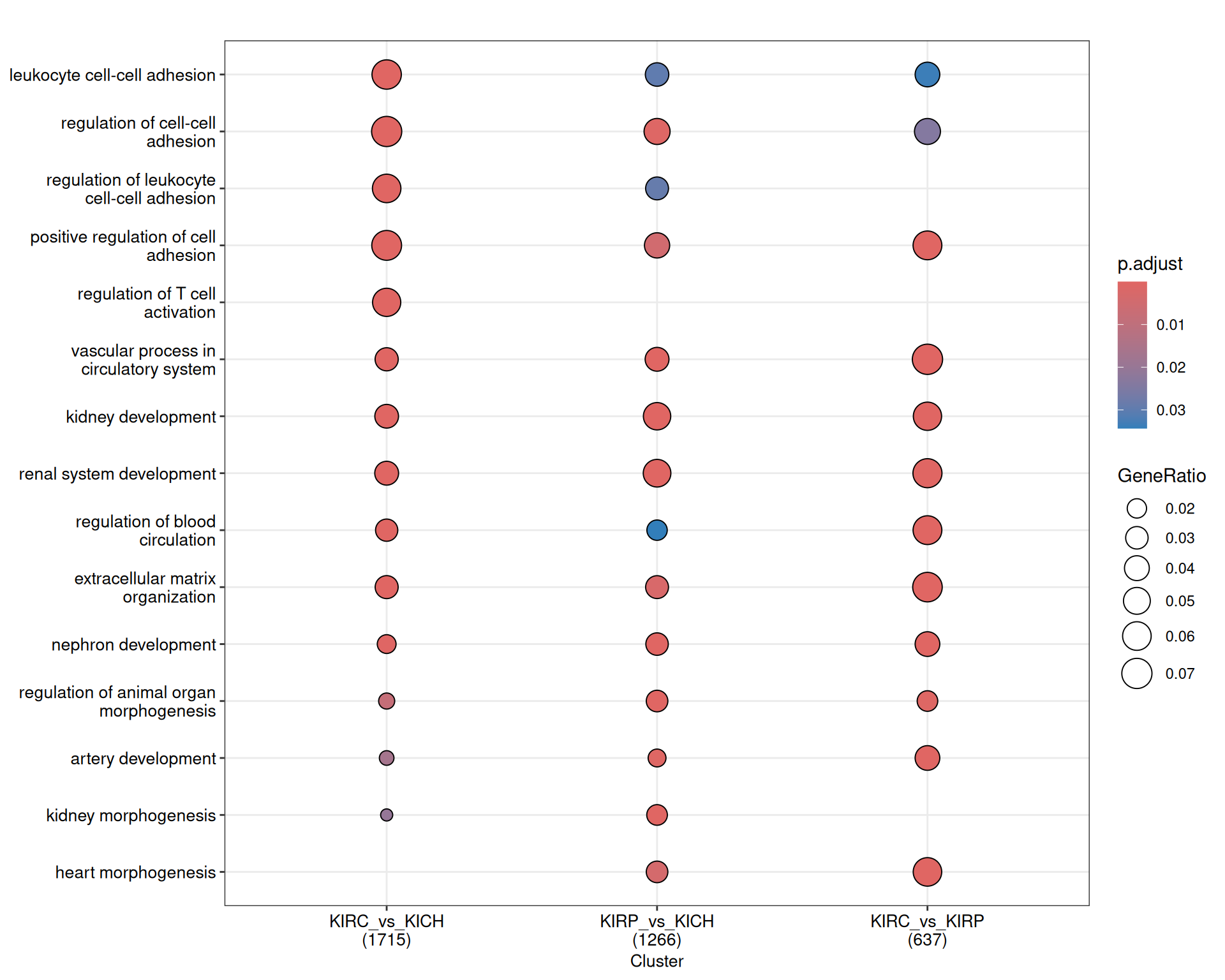
Given the hundreds of genes in each contrast, hundreds of enriched GO BP terms have been identified across the three kidney cancer comparisons: 1,715 in KIRC_vs_KICH, 1,266 in KIRP_vs_KICH and 637 in KIRC_vs_KIRP. The dotplot reports on the most important term for each contrast, and based on this high-level overview we cannot really spot large differences across the three comparisons except for “regulation of T cell activation” that seems to be present only in KIRC_vs_KICH and not in the other contrasts.

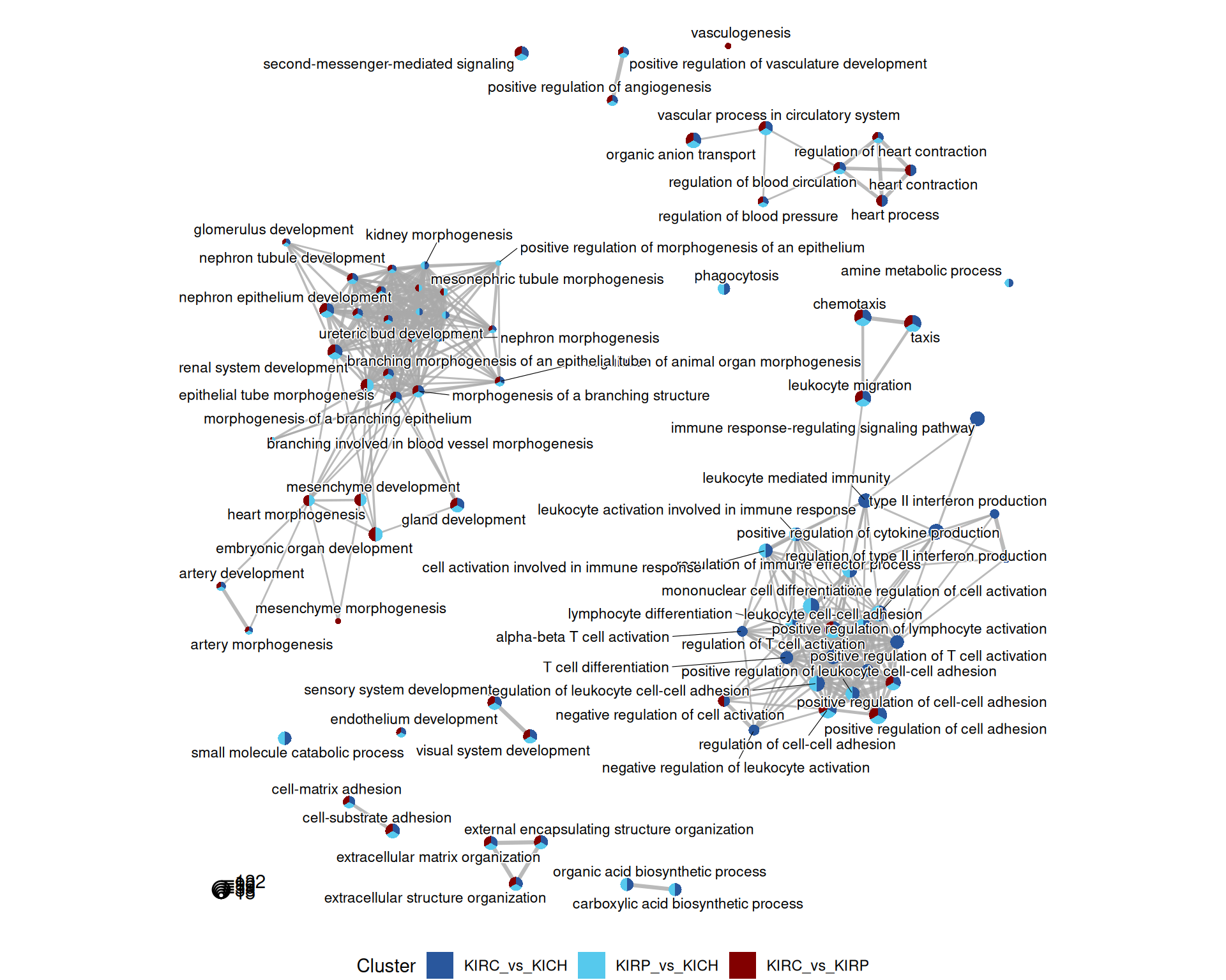
The terms map provides an overview of the relationships between the most significant GO terms, and in which contrasts they appear. Each term is a colored circle, and each connection is a relationship of hierarchy between two terms. Each circle (term) is colored based on the contrast where it appears. Here, we can get a bit more insights in the differences between the three kidney cancers, but there is still an overwhelming abundance of information.

A cluster of terms related to immune response, lymphocyte activation, differentiation and recruitment is clearly visible in the KIRC_vs_KICH and KIRP_vs_KICH comparisons, while it is absent in the contrast KIRC_vs_KIRP.

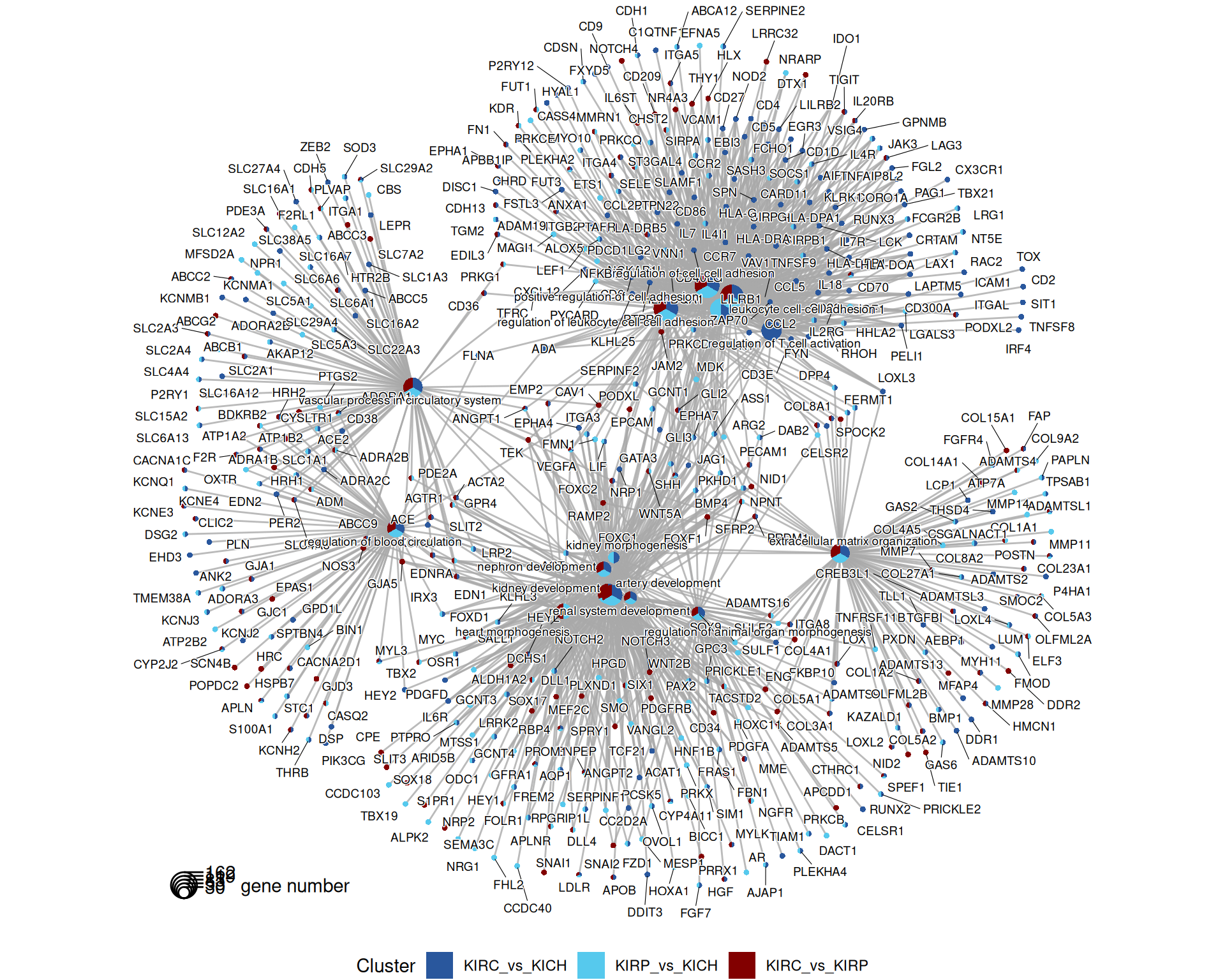
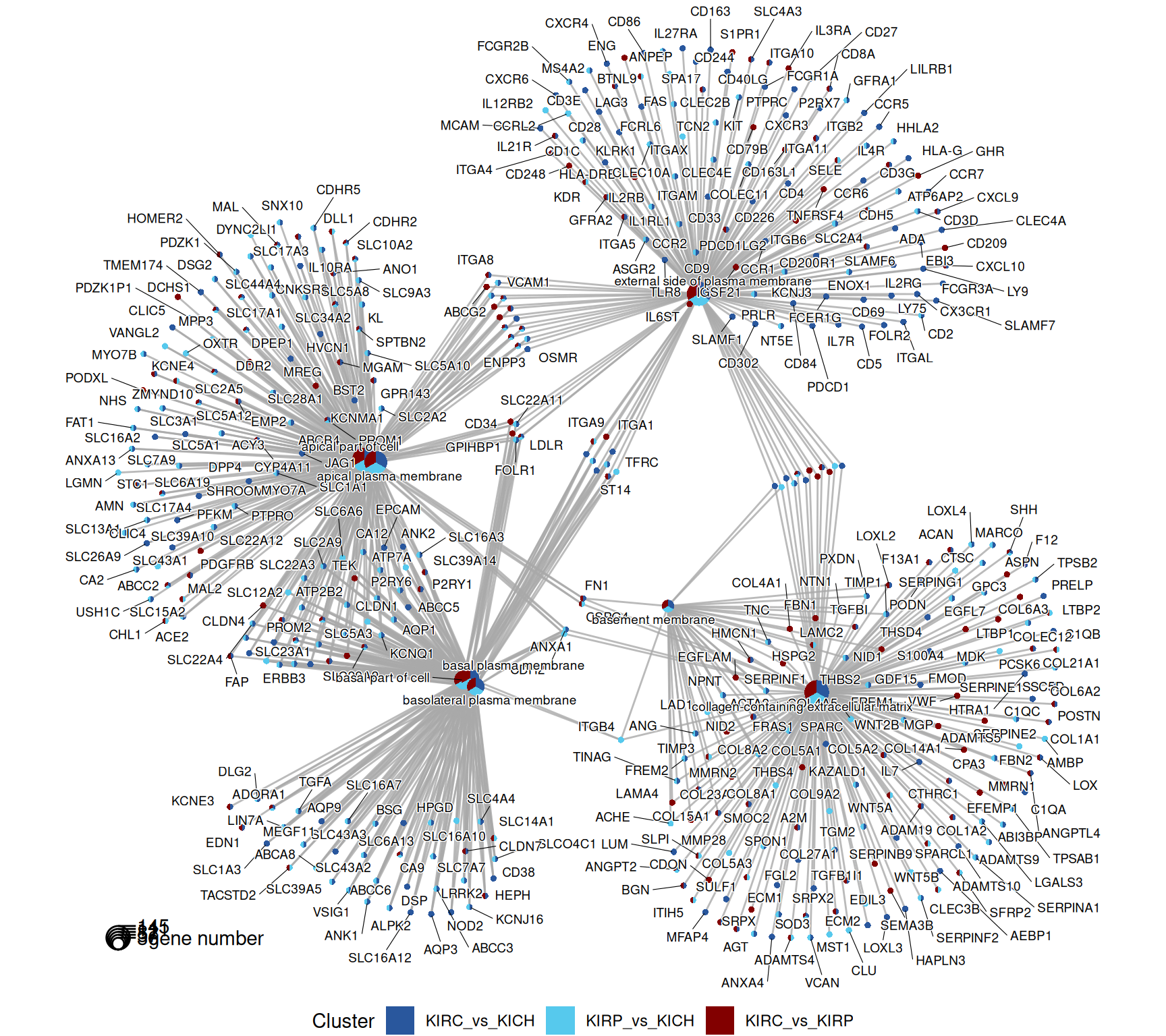
The gene map helps to further refine the genes annotated with the most significant GO terms. Genes are connected to the corresponding GO term, and coloured according to the contrasts that they belong to.

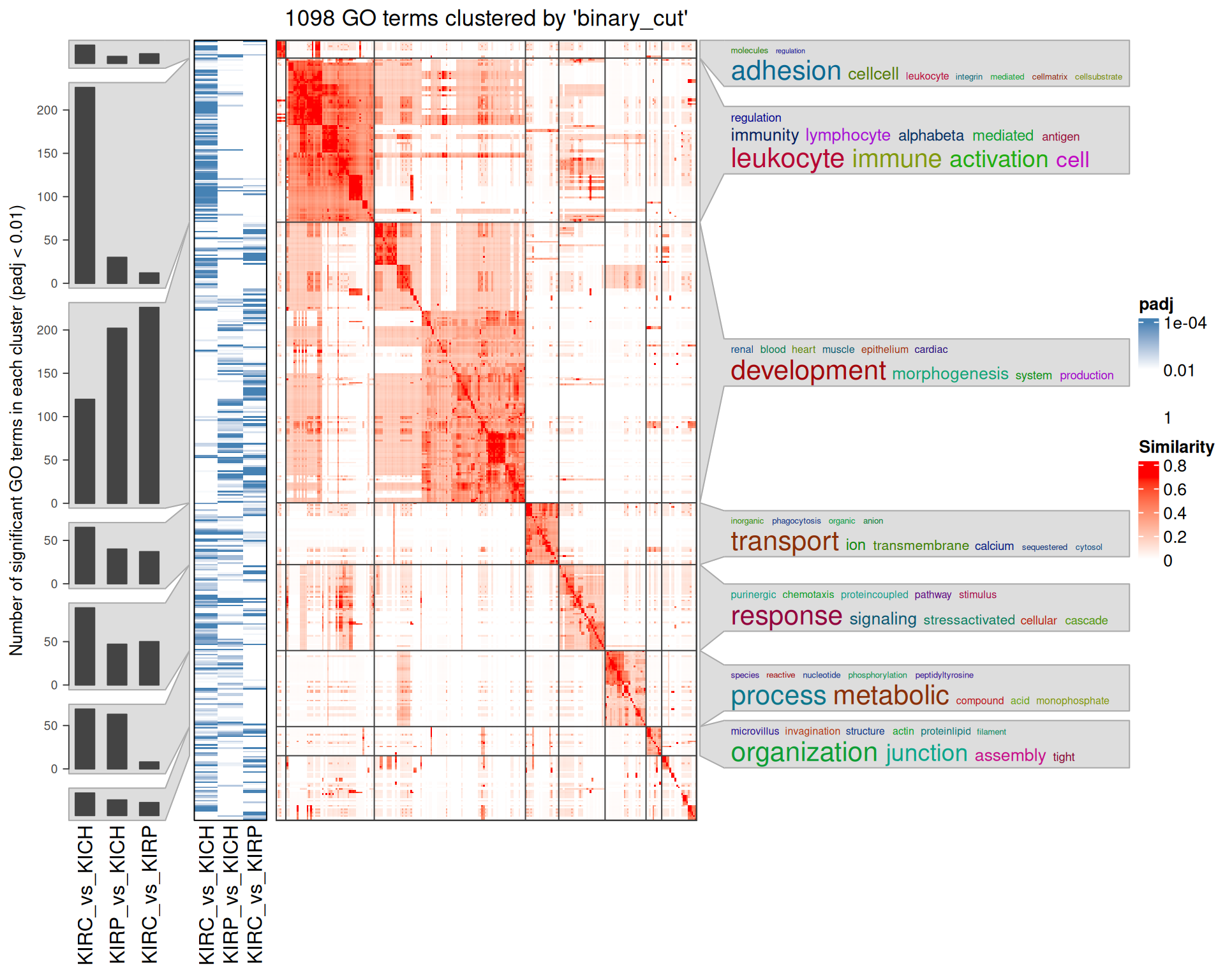
Interpretation of the large amount of GO BP terms identified is difficult, given as well their similarity across the three contrasts. An option to increase interpretability is to cluster the GO terms based on their hierarchy and similarity. An elegant way to do so is to compute a distance matrix of the GO terms, and then perform a binary cut to identify GO terms clusters.

The rich GO cluster heatmap confirms that immune response and leucocyte activation terms are enriched in the KIRC_vs_KICH contrast when compared to KIRP_vs_KICH and KIRC_vs_KIRP. Also angiogenesis and development terms are clustered in two blocks that sees KIRC_vs_KICH in one side and KIRP_vs_KICH and KIRC_vs_KIRP on the other one. Ion transport and metabolic processes are more similar between KIRC_vs_KICH and KIRP_vs_KICH, and this could be a set of biological processes that are similarly disregulated in KIRC and KIRP.

The complete list of 2,632 GO BP terms enriched across the three contrasts is reported below.

2.4.2.2 GO Cellular Compartments terms

Gene Ontology Cellular Compartment serves to capture the cellular location where a molecular function takes place.

Figure 13: dotplot of enriched GO Cellular Compartments terms.

Figure 14: Term maps reporting relationships between GO Cellular Compartments across the different contrasts.

Figure 15: gene maps reporting relationships between GO Cellular Compartments enriched across the different contrasts.

Figure 16: gene maps reporting relationships between GO Cellular Compartments enriched across the different contrasts.

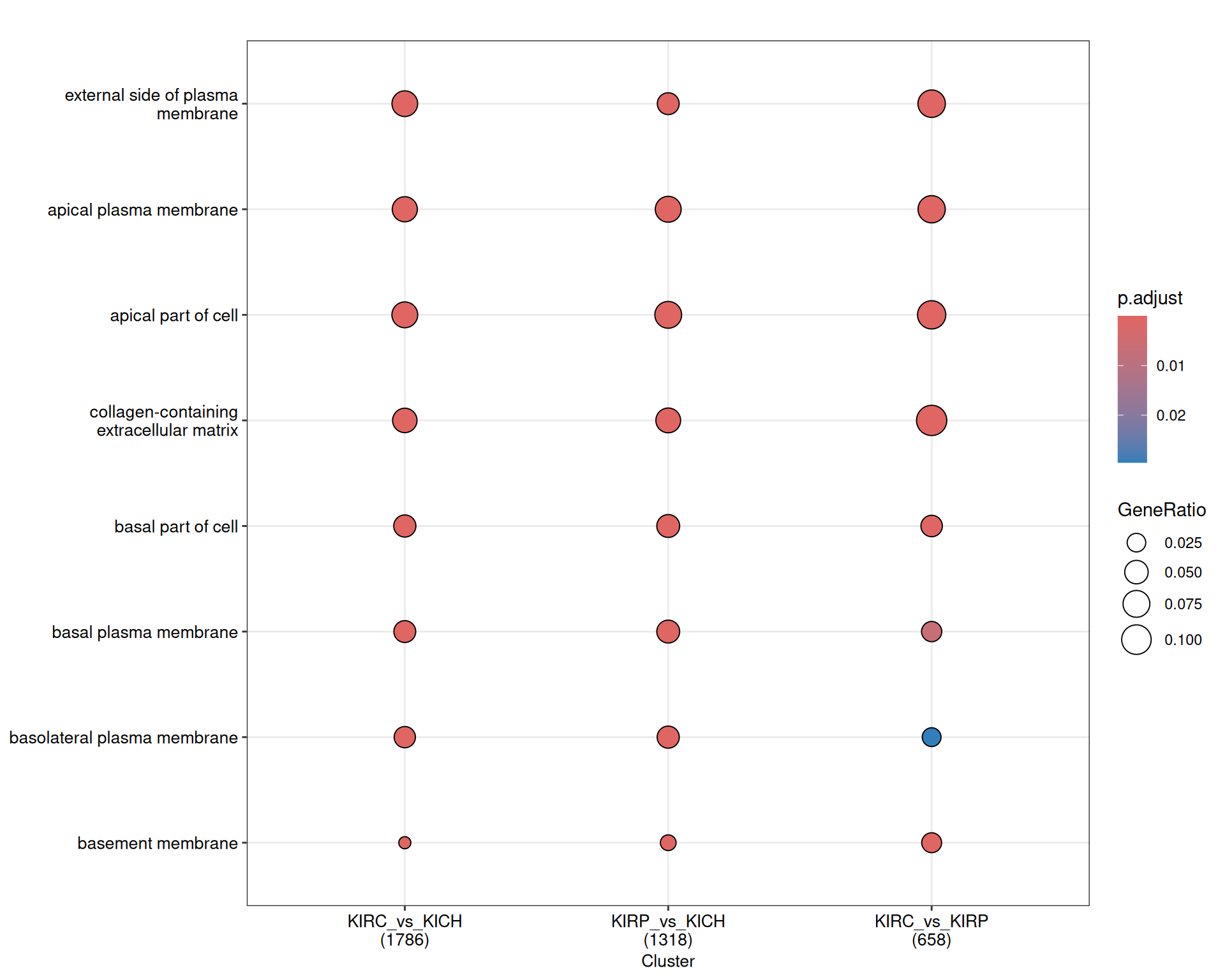
The terms dotplot and indicates that the enriched GO CC terms revolves around “plasma membrane”, “collagen” and the “extra-cellular matrix”, suggesting that most genes that are differentially expressed may be involved in transport across the plasma membrane and the remodeling of the extra-cellular matrix.

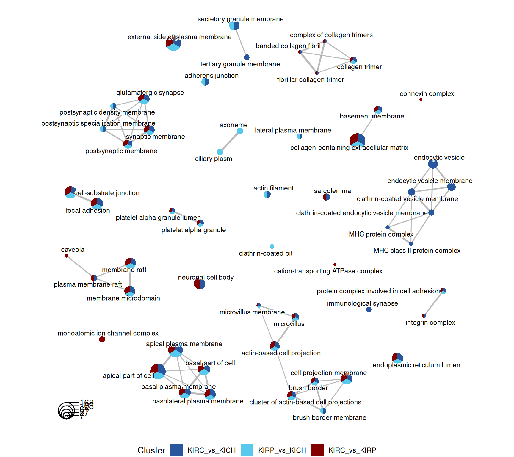
The terms map confirm this message, and in addition we have terms associated with “endocytic vesicles” and “MHC protein complexes” in KIRC_vs_KICH contrast, supporting the idea of a stronger T cell activation in KIRC.

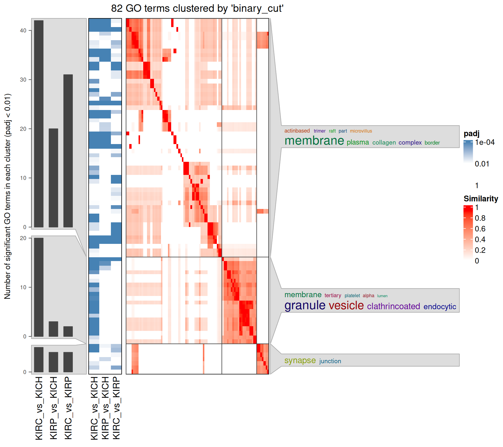
The rich GO cluster heatmap shows that after clustering, most terms associated with plasma membrane and extra-cellular matrix remodeling are more abundant in KIRC_vs_KICH and KIRP_vs_KIRP, suggesting that extra-cellular matrix remodeling is more enhanced in KIRC, and may support a more Epithelial-Mesenchimal Transition (ETM) phenotype of this cancer.

The complete list of 218 GO CC terms enriched across the three contrasts is reported below.

2.4.2.3 GO Molecular Function terms

Gene Ontology Molecular Function serves to represent molecular-level activities performed by gene products.

Figure 17: dotplot of enriched GO Molecular Functions terms.

Figure 18: Term maps reporting relationships between GO Molecular Functions across the different contrasts.

Figure 19: gene maps reporting relationships between GO Molecular Functions enriched across the different contrasts.

Figure 20: gene maps reporting relationships between GO Molecular Functions enriched across the different contrasts.

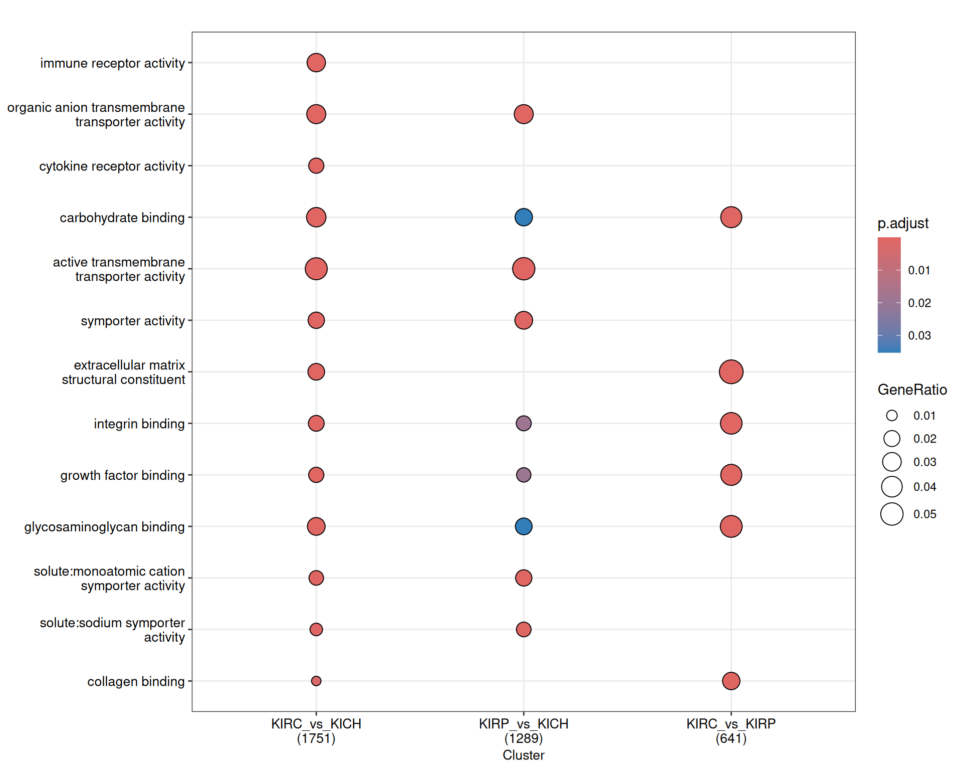
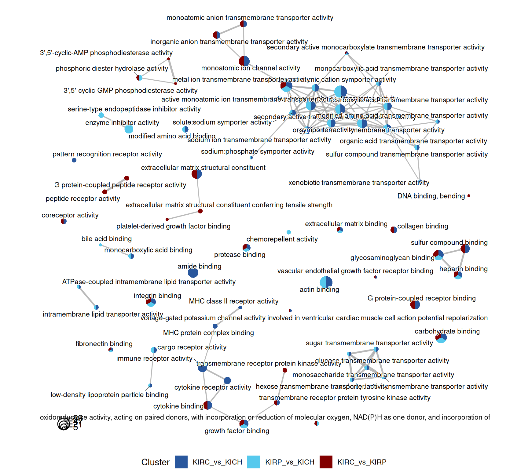
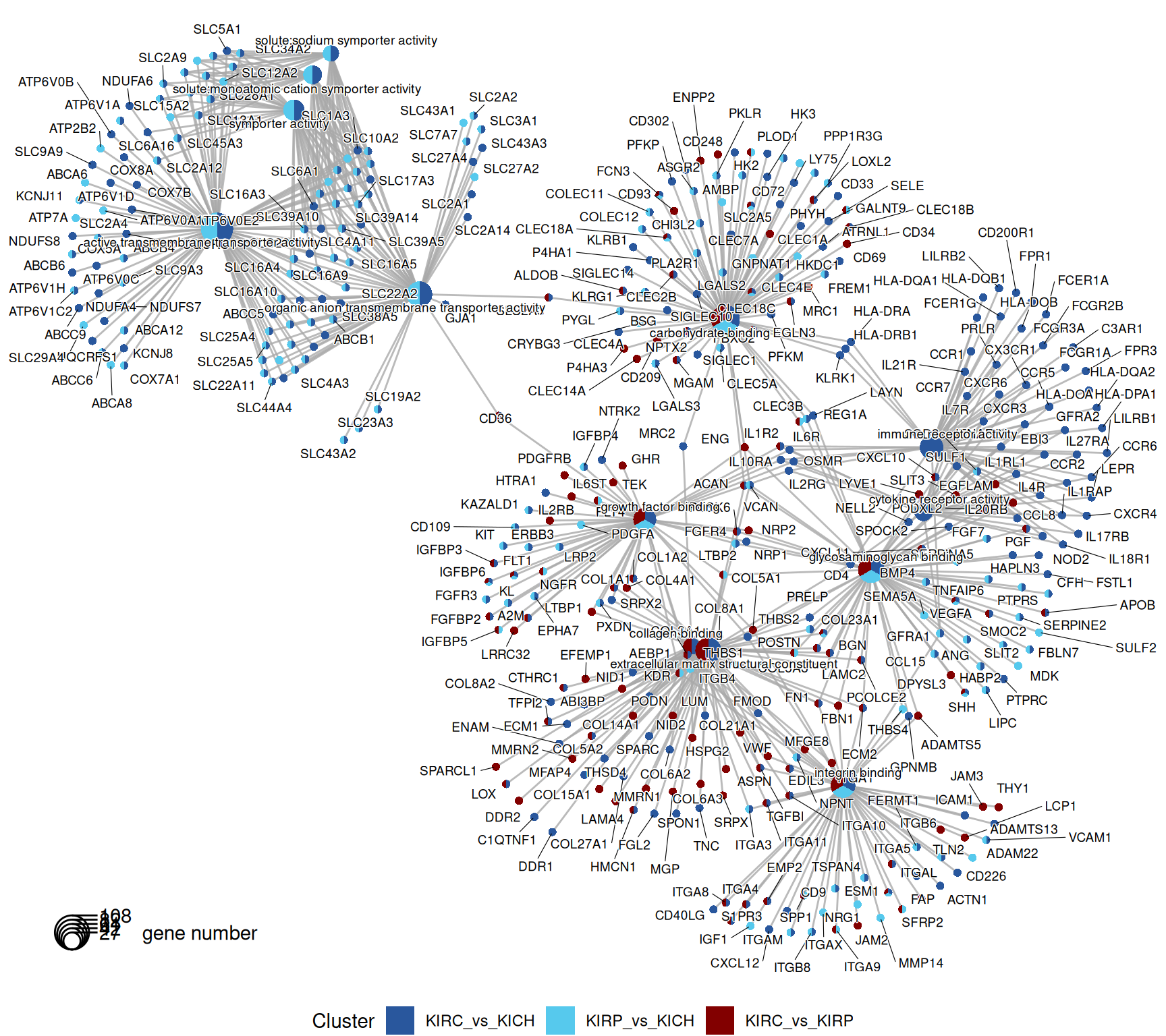
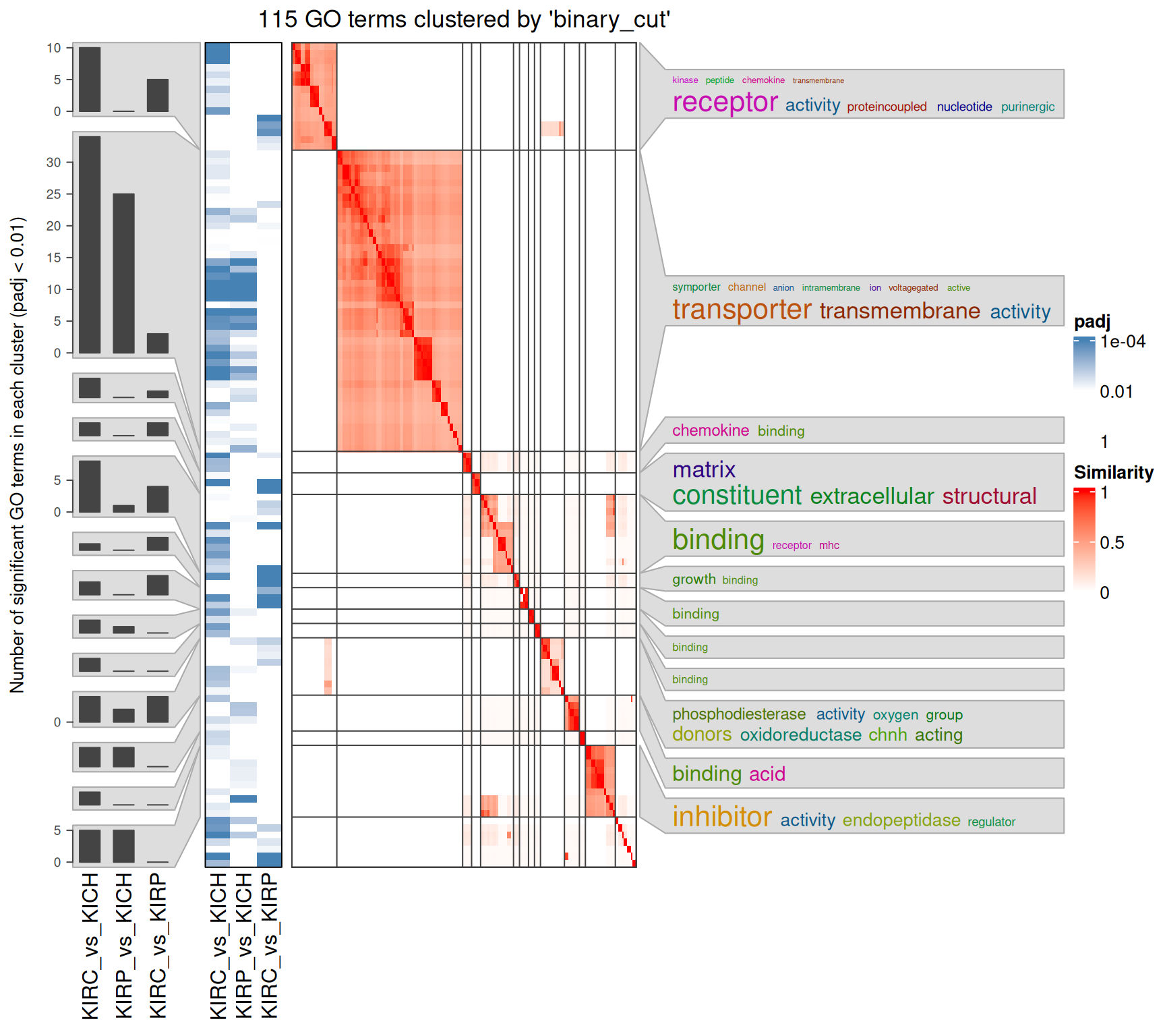
The GO MF terms map and terms cluster suggest clear differences that discriminates KIRC and KICH tumors. KIRC and KIRP seem to have enriched terms on metabolism and strong transporter activities (i.e.: “solute:monoatomic cation symporter activity”, “solute:sodium symporter activity”) when compared to KICH, suggesting that these two kidney cancers are metabolically more active. KIRC instead have enriched GO MF terms associated with remodelling of the extracellular matrix (e.g.: “extracellular matrix structural constituent”, “collagen binding”), receptor activity and chemokine binding (e.g.: “G protein-coupled receptor binding”, “cytokine binding”), suggesting a more hot type of tumor with active recruitment and infiltration of immune cells, when compared to KIRP and KICH.

The complete list of 316 GO MF terms enriched across the three contrasts is reported below.

2.4.2.4 KEGG pathways

KEGG pathways are manually curated and capture our knowledge of the molecular interaction, reaction and relation networks.

Figure 21: dotplot of enriched KEGG pathways.

Figure 22: Term maps reporting relationships between KEGG pathways enriched across the different contrasts.

Figure 23: gene maps reporting relationships between KEGG pathways enriched across the different contrasts.

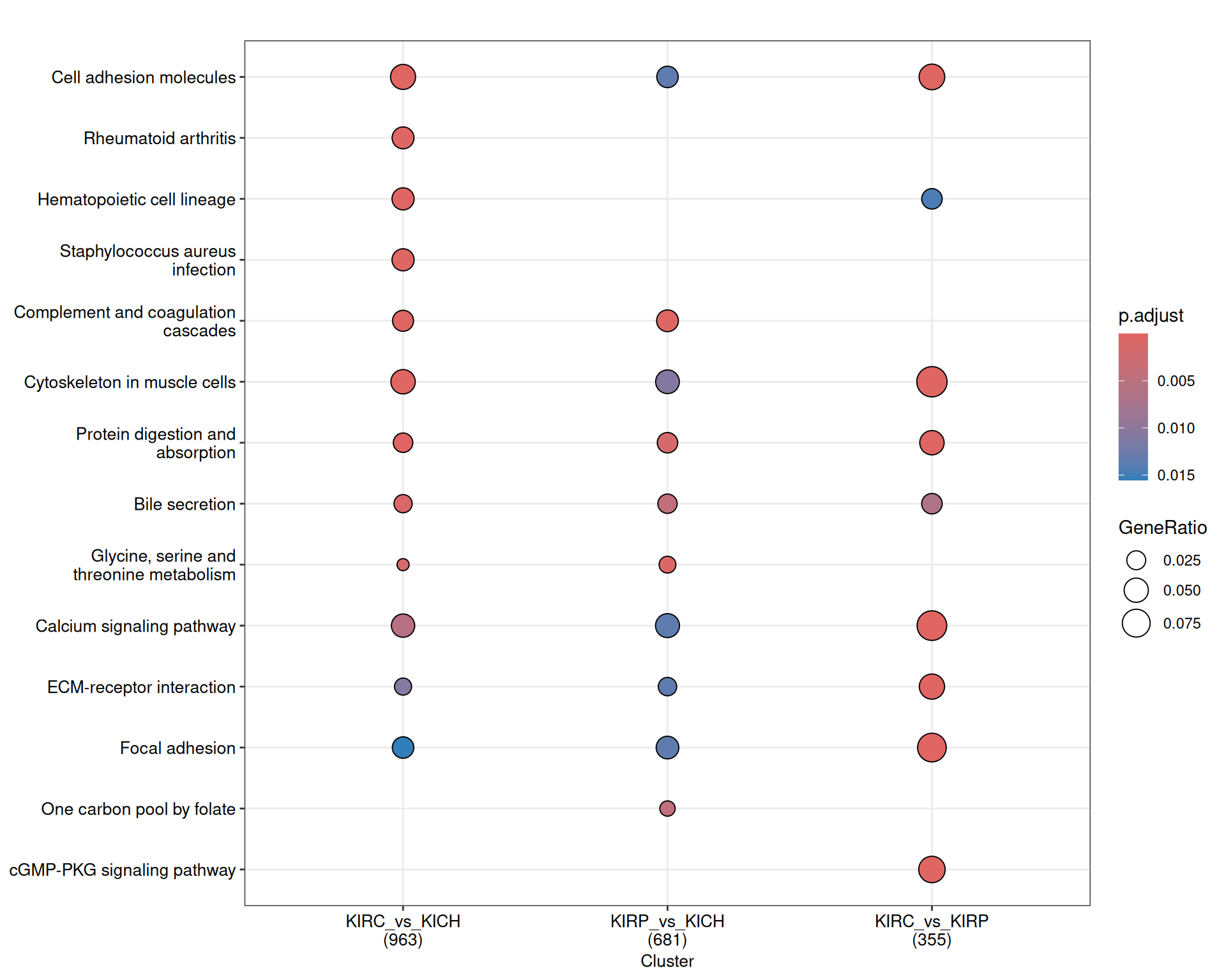
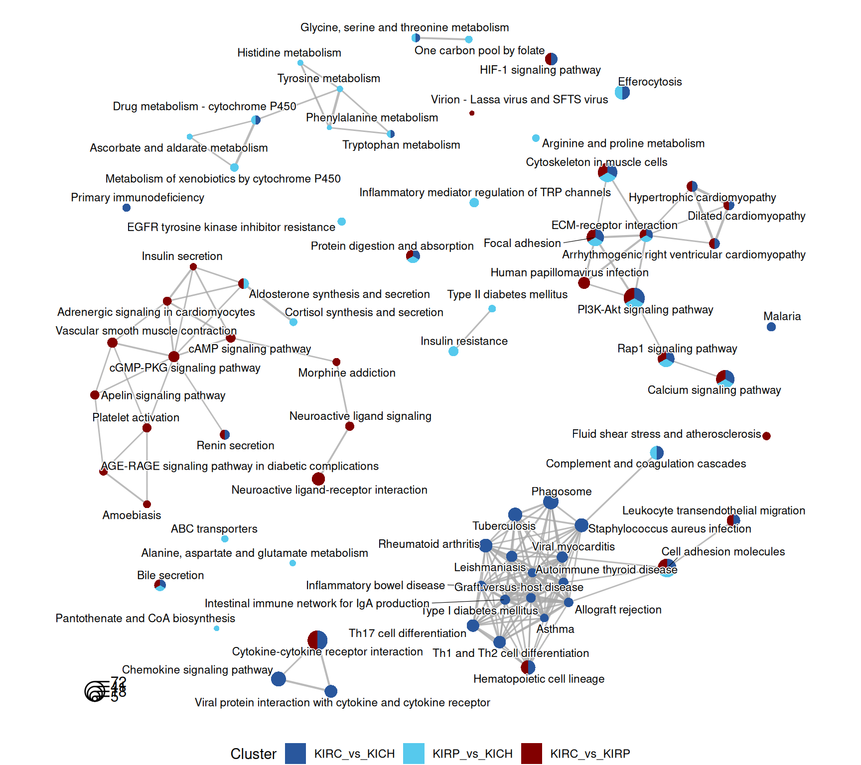
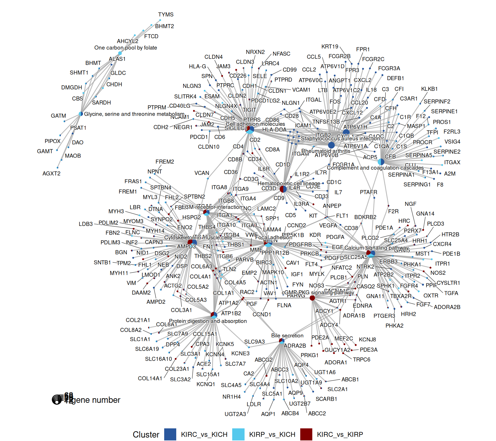
The signal captured in the enriched KEGG pathways seems less clear than the one identified across the enriched GO terms, but in general, the terms maps provide a story in line to what described with the enriched GO terms. KIRC present a stronger immune response when compared to KIRP and KICH (i.e.: “Th1 and Th2 cell differentiation”, “Th17 cell differentiation”, “Hematopoietic cell lineage”) and extracellular matrix remodelling / epithelial-to-mesenchimal transition (e.g.: “Rap1 signaling pathway”).

The complete list of 95 KEGG pathways across the three contrasts is reported below.

2.4.2.5 Reactome pathways

Similarly to KEGG, Reactome pathways are manually curated biological pathways.

Figure 24: dotplot of enriched Reactome pathways.

Figure 25: Term maps reporting relationships between Reactome pathways enriched across the different contrasts.

Figure 26: gene maps reporting relationships between Reactome pathways enriched across the different contrasts.

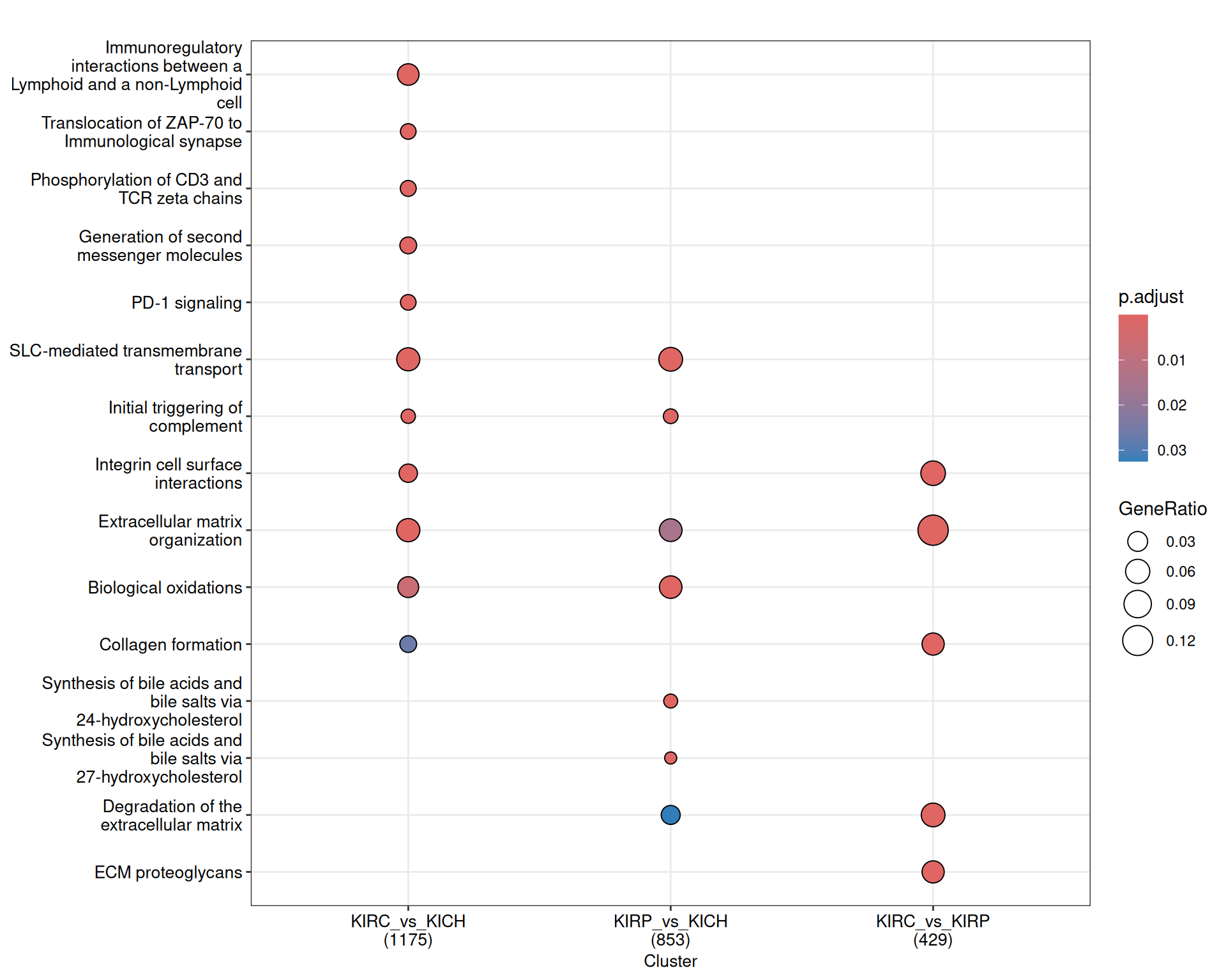
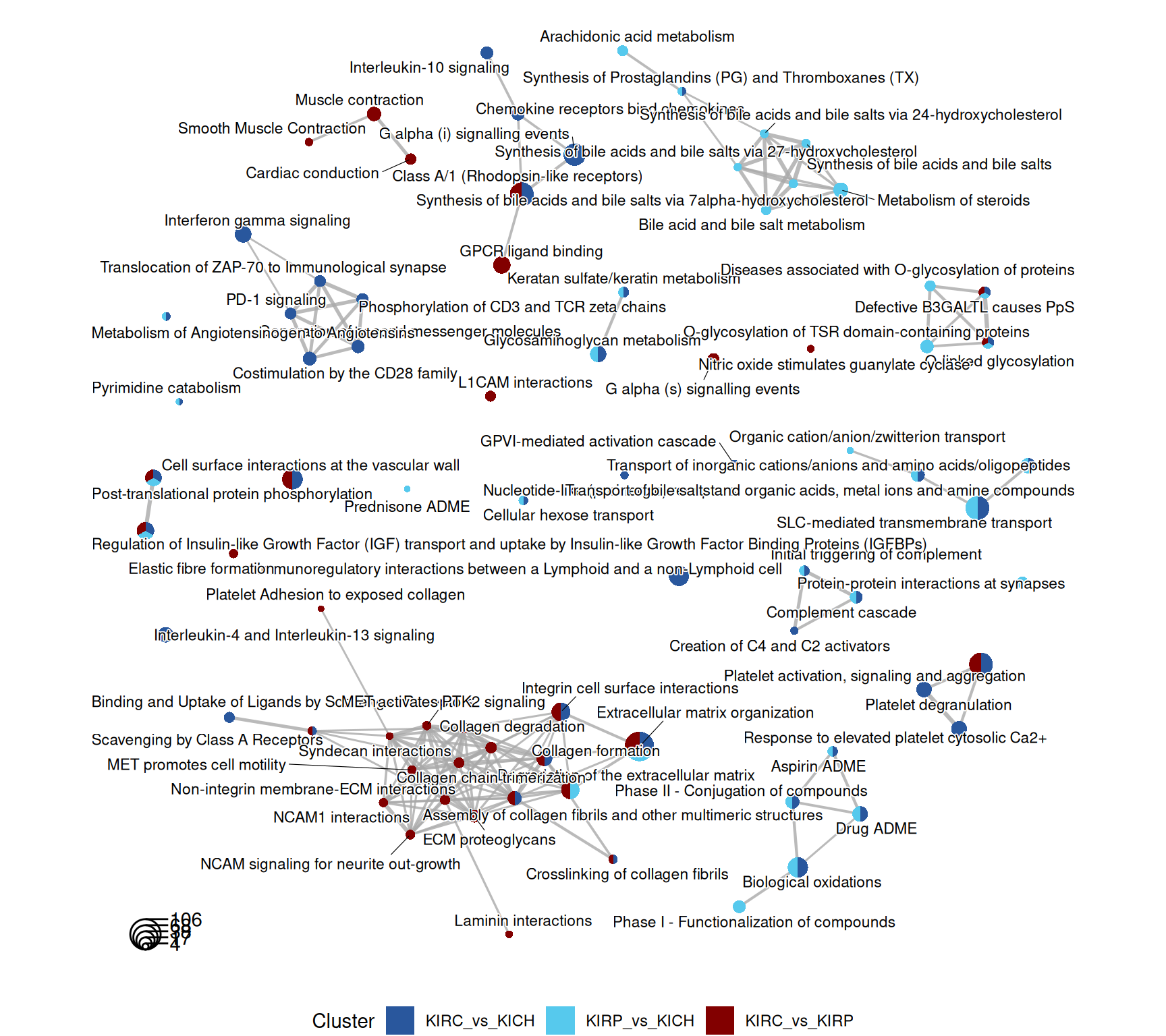
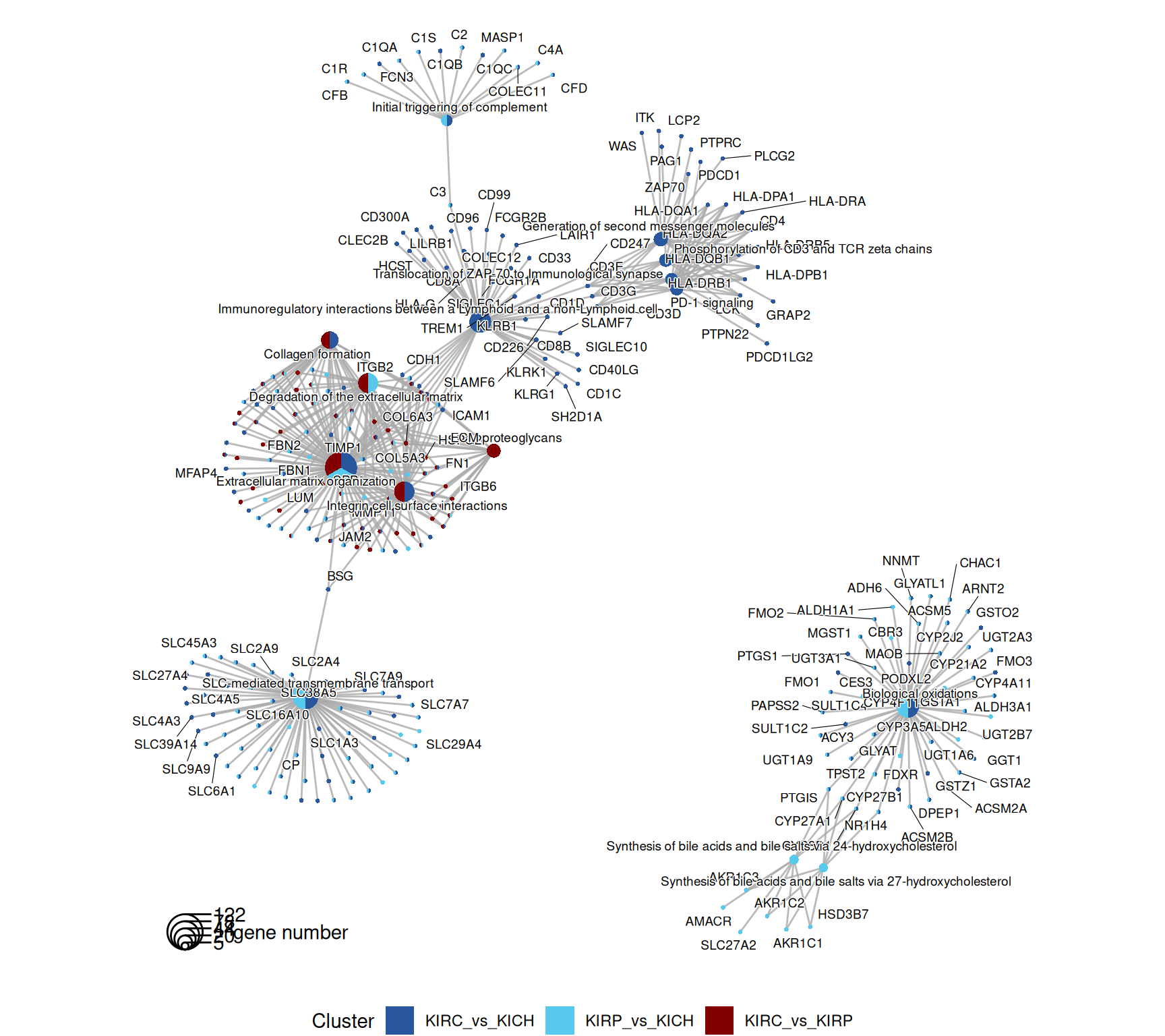
The enriched Reactome pathways are concordant to what emerged so far of the differences and similaritiesof the expression profiles of KIRC, KIRP and KICH kidney carcinomas. KIRC and KIRP have enriched pathwasy related to ion transports and metabolism (e.g.: “SLC-mediated transmembrane transport”, “glycosaminoglycan metabolism”, “biological oxidations”). KIRP has disregulated fatty acid metabolism (“metabolism of steroids”, “synthesis of bile acids and bile salts”), while KIRC has a strong immune engagement (“Costimulation by CD28 family”, “PD-1 signaling”, “Phosphorylation of CD3 and TCR zeta chains”) and extracellular matrix remodelling (“MET promotes cell motility”, “NCAM1 interactions”, “Non-integrin membrane-ECM interactions”)

The complete list of 154 Reactome pathways enriched across the three contrasts is reported below.

2.4.2.6 WikiPathways

Lastly, also WikiPathways provides another angle on a set of manually curated biological pathways.

Figure 27: dotplot of enriched Wikipathways pathways.

Figure 28: Term maps reporting relationships between WikiPathways enriched across the different contrasts.

Figure 29: gene maps reporting relationships between WikiPathways enriched across the different contrasts.

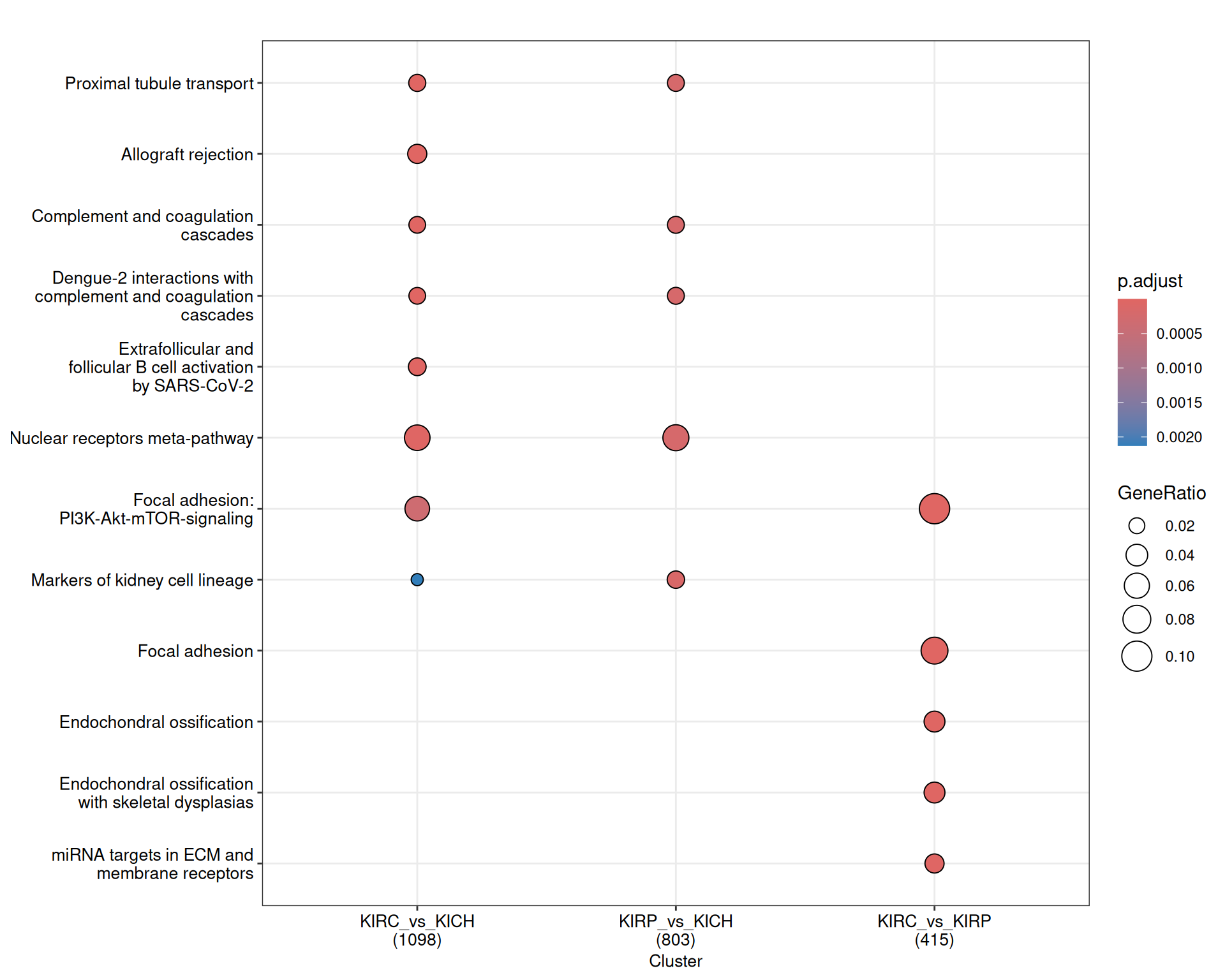
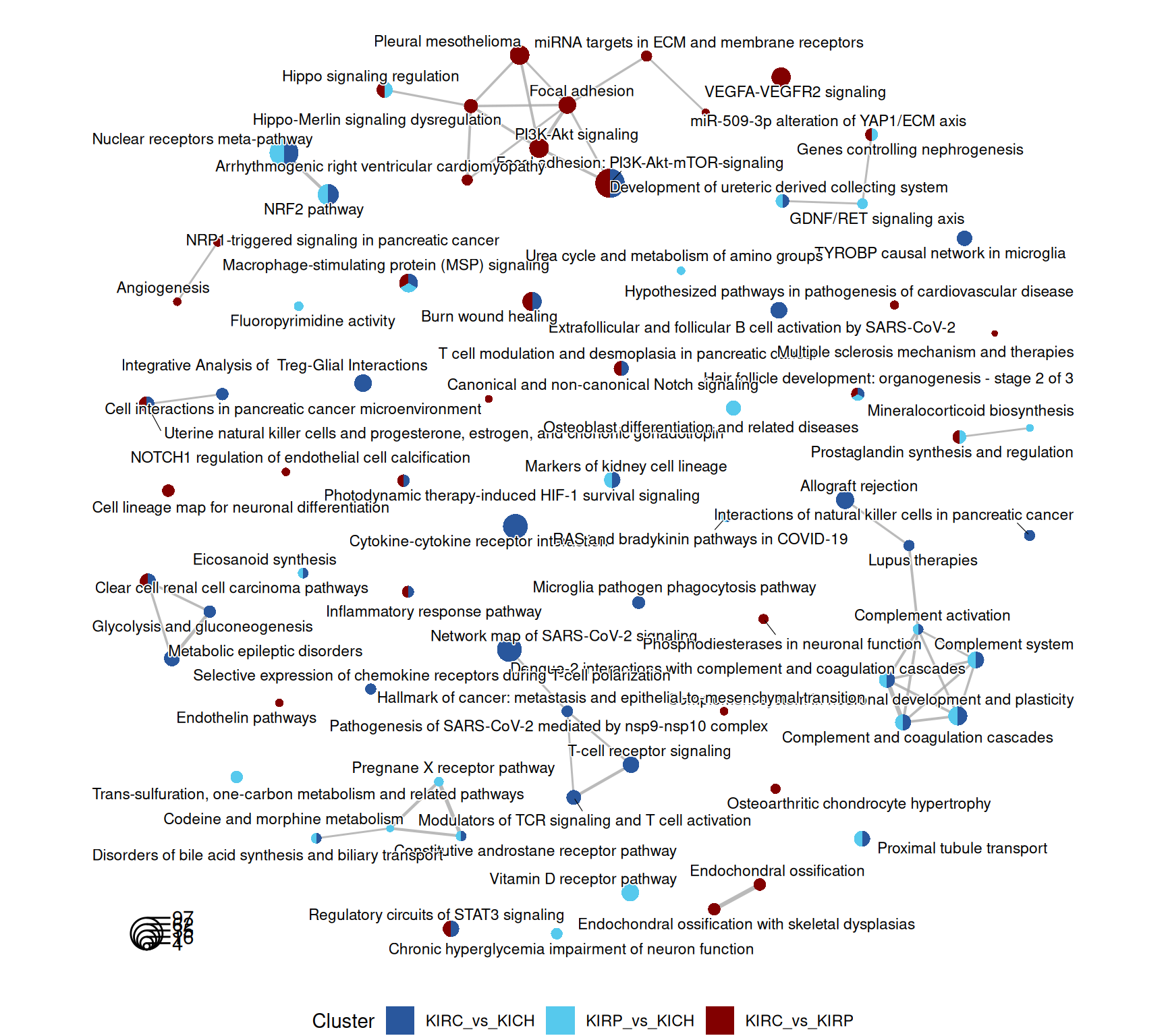
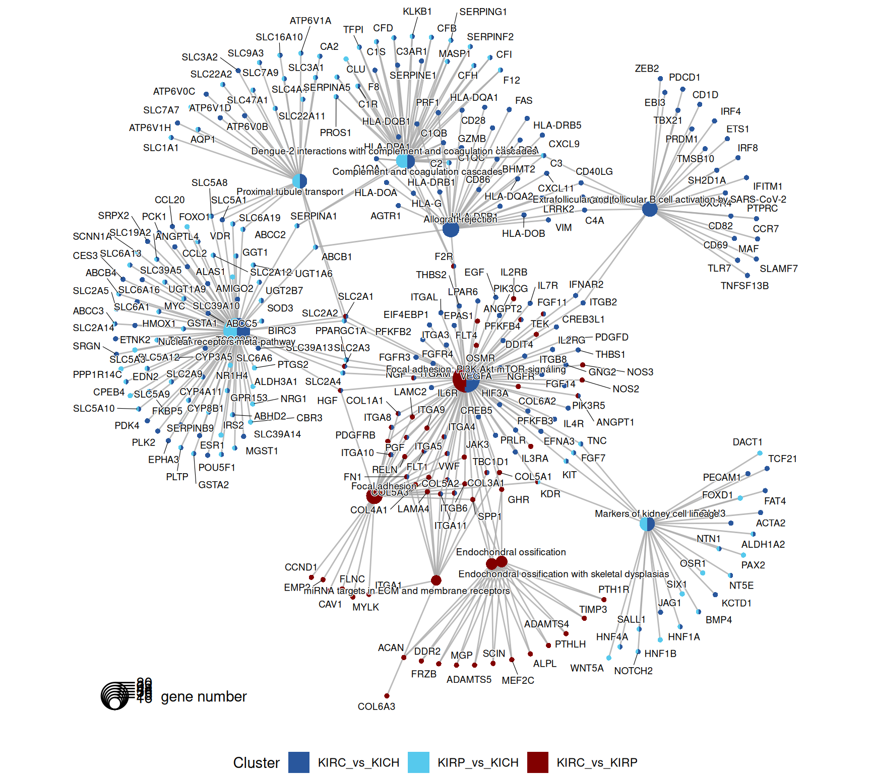
The enriched WikiPathways are consistent with the biological signals captured so far. KIRC and KIRP have enriched metabolism and ion transporters (“Proximal tubule transport”) when compared to KICH. KIRC has a strong signature of immune activation (“Inflammatory response pathway”, “Modulator of TCR signaling and T cell activation”, “T-cell receptor signaling”) and ECM remodelling (“Focal adhesion: PI3K-Akt-mTOR signaling”, “miRNAs targets in ECM and membrane receptors”).

The complete list of 154 WikiPathways pathways enriched across the three contrasts is reported below.

2.5 Infiltrating immune cells

The Gene Set Enrichment Analyses (Section 2.4.2) revealed that immune response and immune cells infiltration is an emerging biological theme in KIRC when compared to KIRP and KICH kidney carcinomas. While for TCGA we do not have single-cell datasets that would allow for a precise quantification and characterization of the tumor micro-environment, we can get an approximate view of the differences in infiltrating immune cells between the three kidney carcinomas by looking at bulk RNA-seq cellular deconvolution techniques.

For this, I will use the R package infiltR, which includes three common bulk RNA-seq deconvolution tools for quantification of tumor-infiltrating immune cells:

infiltR uses MCP-counter to obtain absolute quantification of infiltrating immune cells, while a more detailed profiling of relative immune cells subtypes is performed with CIBERSORT and quanTIseq.

Let’s look at the main output of the infiltR predictions:

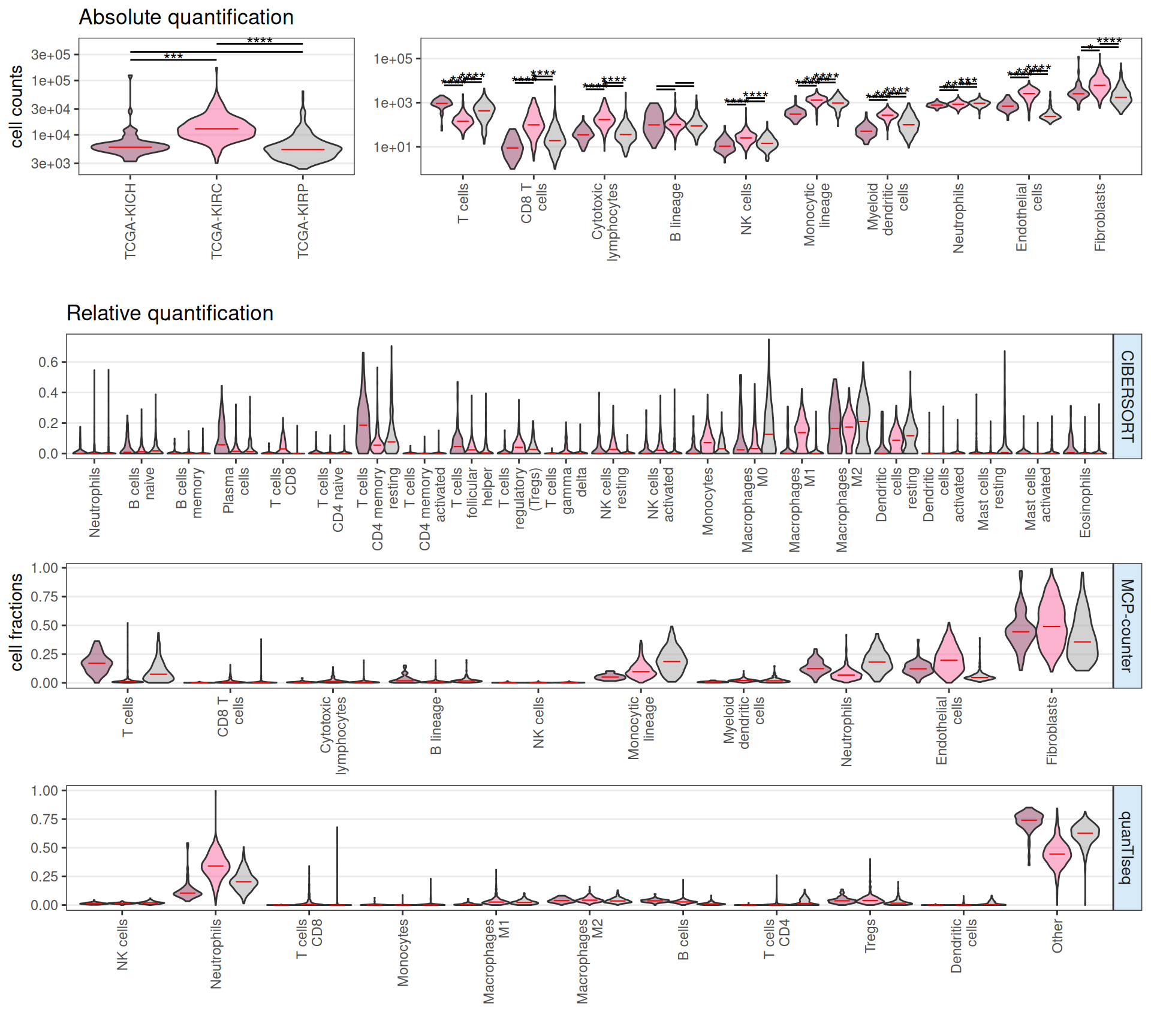
Figure 30: Infiltraing immune cells estimates.

On the top panel we have the absolute quantification as estimated by MCP-counter, while in the bottom panel we have the relative quantification based on CIBERSORT, MCP-counter and quanTIseq. The emerging picture on the infilatring immune cells is consistent with the enriched pathways we have identified with the GSEA analysis:

KICH: KICH appears like a “cold” tumor, with less infiltrating immune cells, if compared to KIRC and KIRP. Limited immune engagement may limit the number of possible immune-therapeutic targets.
- KICH has less absolute number of infiltrating immune cells than KIRC, and similar to KIRP.
- KICH has more T CD4 memory cells and less Tregs fractions than KIRC and KIRP.
- KICH has less Neutrophils, Monocytes and Macrophages fractions than KIRC and KIRP.
KIRC: KIRC appears to have a high amount of infiltrating immune cells. The proportion between CD8 T cells and Tregs may indicate an immune-inflamed but immunosuppressed microenvironment, supported as well by the presence of monocytes and macrophages
- KIRC has the highest count of total infiltrating immune cells, and the highest count of CD8 T cells.
- KIRC has the highest fraction of CD8 T cells and Tregs.
- KIRC has the highest fraction of infiltrating monocytes and macrophages M1, and high fraction of Macrophages 2 and Dendritic cells.
KIRP: KIRP appears to have an immature macrophage population in the tumor microenvironment. These M0 macrophages may polarize into either M1 (pro-inflammatory) or M2 (immunosuppressive).
- KIRP has an absolute count of infiltrating immune cells comparable to KICH.
- KIRP cell fractions contains the highest Macrophages M0, Macrophages M2 and Dendritic cells resting.
- KIRP cell fraction contains high Tregs.

In Figure 31 we can spot some discrepancies between the predicted infiltrating immune cells proportion across the different methods. infiltR allows as well to compare check the concordance between different estimates, by performing a pairwise aggregation the immune cell types and compare them across couples of methods.

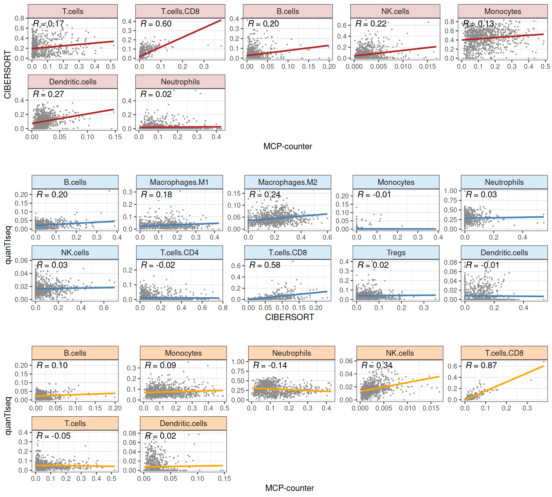
Figure 31: Concordance between different estimates.

The sanity-check plot in Figure 32 reveals that except for the CD8 T cells estimates, the estimates of the three methods have poor correlation. This can be ascribed to the different underlying algorithms for the three different methods, with different assumptions, strengths and weaknesses. Moreover, the overall overlap between cell types detected (more granular for CIBERSORT, more general for MCP-counter) is low, and infiltR aggregation to the minimum-common denominator to perform the comparison may enhance the discrepancy between the methodologies.

2.6 Lessons Learnt

Based on transcriptomics data, we have learnt:

Exploratory analysis suggests:
- KICH clusters with KIRP based on gene expression data.
- Little to no correlation with vital status or residual disease (follow up tumor status) with kidney carcinoma types.
Differential Gene Expression analysis:
- here KIRC and KIRP seems more similar to each other (946 DGE genes in common vs KICH).
- KIRC vs KICH enriched in terms associated immune response, T-cell activation, lymphocyte recruitment and stress signaling cascades.
- KIRC seems to have KEGG pathways associated with tumor promoting inflammation, cell proliferation, invasion and metastasis.
Tumor-microenvironment characterization:
- KICH appears like a “cold” tumor, with less infiltrating immune cells, if compared to KIRC and KIRP.
- KIRC appears to have a high amount of infiltrating immune cells, with an immune-inflamed but immunosuppressed microenvironment.

2.7 Session Information

Note

R version 4.3.3 (2024-02-29)
Platform: x86_64-pc-linux-gnu (64-bit)
Running under: Ubuntu 24.04.3 LTS

Matrix products: default
BLAS:   /usr/lib/x86_64-linux-gnu/blas/libblas.so.3.12.0 
LAPACK: /usr/lib/x86_64-linux-gnu/lapack/liblapack.so.3.12.0

locale:
 [1] LC_CTYPE=en_US.UTF-8    LC_NUMERIC=C            LC_TIME=C              
 [4] LC_COLLATE=en_US.UTF-8  LC_MONETARY=C           LC_MESSAGES=en_US.UTF-8
 [7] LC_PAPER=C              LC_NAME=C               LC_ADDRESS=C           
[10] LC_TELEPHONE=C          LC_MEASUREMENT=C        LC_IDENTIFICATION=C    

time zone: Europe/Brussels
tzcode source: system (glibc)

attached base packages:
[1] grid      stats4    stats     graphics  grDevices utils     datasets 
[8] methods   base     

other attached packages:
 [1] UpSetR_1.4.0              umap_0.2.10.0            
 [3] stringr_1.5.1             simplifyEnrichment_1.12.0
 [5] scales_1.4.0              RColorBrewer_1.1-3       
 [7] PCAtools_2.14.0           org.Hs.eg.db_3.18.0      
 [9] matrixStats_1.5.0         infiltR_0.1.0            
[11] gridExtra_2.3             forcats_1.0.0            
[13] EnhancedVolcano_1.20.0    ggrepel_0.9.6            
[15] ggplot2_3.5.2             edgeR_4.0.16             
[17] limma_3.58.1              DT_0.33                  
[19] dplyr_1.1.4               DOSE_3.28.2              
[21] data.table_1.17.8         cowplot_1.2.0            
[23] clusterProfiler_4.10.1    BiocSingular_1.18.0      
[25] BiocParallel_1.36.0       AnnotationDbi_1.64.1     
[27] IRanges_2.36.0            S4Vectors_0.40.2         
[29] Biobase_2.62.0            BiocGenerics_0.48.1      

loaded via a namespace (and not attached):
  [1] fs_1.6.6                    bitops_1.0-9               
  [3] enrichplot_1.22.0           lubridate_1.9.4            
  [5] HDO.db_0.99.1               httr_1.4.7                 
  [7] doParallel_1.0.17           tools_4.3.3                
  [9] backports_1.5.0             R6_2.6.1                   
 [11] mgcv_1.9-1                  lazyeval_0.2.2             
 [13] GetoptLong_1.0.5            withr_3.0.2                
 [15] graphite_1.48.0             preprocessCore_1.64.0      
 [17] quantreg_6.1                cli_3.6.5                  
 [19] scatterpie_0.2.5            labeling_0.4.3             
 [21] slam_0.1-55                 sass_0.4.10                
 [23] S7_0.2.0                    tm_0.7-16                  
 [25] proxy_0.4-27                askpass_1.2.1              
 [27] yulab.utils_0.2.0           gson_0.1.0                 
 [29] dichromat_2.0-0.1           RSQLite_2.4.2              
 [31] RApiSerialize_0.1.4         generics_0.1.4             
 [33] gridGraphics_0.5-1          shape_1.4.6.1              
 [35] crosstalk_1.2.1             car_3.1-3                  
 [37] GO.db_3.18.0                Matrix_1.6-5               
 [39] abind_1.4-8                 lifecycle_1.0.4            
 [41] yaml_2.3.10                 carData_3.0-5              
 [43] ggpmisc_0.6.2               SummarizedExperiment_1.32.0
 [45] MCPcounter_1.2.0            qvalue_2.34.0              
 [47] SparseArray_1.2.4           blob_1.2.4                 
 [49] dqrng_0.4.1                 crayon_1.5.3               
 [51] lattice_0.22-5              beachmat_2.18.1            
 [53] KEGGREST_1.42.0             pillar_1.11.0              
 [55] knitr_1.50                  ComplexHeatmap_2.18.0      
 [57] fgsea_1.35.6                GenomicRanges_1.54.1       
 [59] rjson_0.2.23                lpSolve_5.6.23             
 [61] codetools_0.2-19            fastmatch_1.1-6            
 [63] glue_1.8.0                  ggfun_0.2.0                
 [65] vctrs_0.6.5                 png_0.1-8                  
 [67] treeio_1.26.0               gtable_0.3.6               
 [69] ggpp_0.5.9                  cachem_1.1.0               
 [71] xfun_0.52                   limSolve_2.0.1             
 [73] S4Arrays_1.2.1              tidygraph_1.3.1            
 [75] survival_3.8-3              iterators_1.0.14           
 [77] statmod_1.5.0               nlme_3.1-164               
 [79] ggtree_3.10.1               bit64_4.6.0-1              
 [81] GenomeInfoDb_1.38.8         bslib_0.9.0                
 [83] irlba_2.3.5.1               colorspace_2.1-1           
 [85] DBI_1.2.3                   tidyselect_1.2.1           
 [87] proxyC_0.5.2                bit_4.6.0                  
 [89] compiler_4.3.3              graph_1.80.0               
 [91] SparseM_1.84-2              xml2_1.3.8                 
 [93] NLP_0.3-2                   DelayedArray_0.28.0        
 [95] stringfish_0.17.0           shadowtext_0.1.5           
 [97] quadprog_1.5-8              rappdirs_0.3.3             
 [99] digest_0.6.37               rmarkdown_2.29             
[101] XVector_0.42.0              htmltools_0.5.8.1          
[103] pkgconfig_2.0.3             sparseMatrixStats_1.14.0   
[105] MatrixGenerics_1.14.0       fastmap_1.2.0              
[107] rlang_1.1.6                 GlobalOptions_0.1.2        
[109] htmlwidgets_1.6.4           DelayedMatrixStats_1.24.0  
[111] farver_2.1.2                jquerylib_0.1.4            
[113] jsonlite_2.0.0              GOSemSim_2.28.1            
[115] RCurl_1.98-1.17             magrittr_2.0.3             
[117] polynom_1.4-1               Formula_1.2-5              
[119] GenomeInfoDbData_1.2.11     ggplotify_0.1.2            
[121] patchwork_1.3.1             Rcpp_1.1.0                 
[123] ggnewscale_0.5.2            ape_5.8-1                  
[125] viridis_0.6.5               reticulate_1.43.0          
[127] stringi_1.8.7               ggraph_2.2.1               
[129] zlibbioc_1.48.2             MASS_7.3-60.0.1            
[131] plyr_1.8.9                  parallel_4.3.3             
[133] doSNOW_1.0.20               Biostrings_2.70.3          
[135] graphlayouts_1.2.2          splines_4.3.3              
[137] circlize_0.4.16             locfit_1.5-9.12            
[139] igraph_2.1.4                reshape2_1.4.4             
[141] ScaledMatrix_1.10.0         evaluate_1.0.4             
[143] quantiseqr_1.10.0           RcppParallel_5.1.10        
[145] BiocManager_1.30.26         foreach_1.5.2              
[147] tweenr_2.0.3                MatrixModels_0.5-4         
[149] tidyr_1.3.1                 openssl_2.3.3              
[151] purrr_1.1.0                 polyclip_1.10-7            
[153] qs_0.27.3                   clue_0.3-66                
[155] ReactomePA_1.46.0           ggforce_0.5.0              
[157] rsvd_1.0.5                  broom_1.0.9                
[159] reactome.db_1.86.2          e1071_1.7-16               
[161] RSpectra_0.16-2             tidytree_0.4.6             
[163] rstatix_0.7.2               viridisLite_0.4.2          
[165] class_7.3-22                snow_0.4-4                 
[167] tibble_3.3.0                aplot_0.2.8                
[169] memoise_2.0.1               cluster_2.1.6              
[171] timechange_0.3.0