4 micro-RNAs Analysis
4.1 On this page
Biological insights and take-home messages are at the bottom of the page at Lesson Learnt: Section 4.5.
- Here we investigate the micro-RNAs data across the three Kidney Cancers.
- First we filter lowly expressed micro-RNAs and we do some exploratory analyses on samples, micro-RNAs expression and clinical covariates.
- We then run a formal Differential Gene Expression analysis to identify micro-RNAs that have different expression levels across the three Kidney cancer types.
4.2 micro-RNAs data overview and QC
4.2.1 micro-RNAs counts overview
For TCGA Kidney cancer micro-RNAs data, we will perform analyses similar to the ones performed for the transcriptomics one (see Chapter 2) and proteomics (see Chapter 3). We first start with an overview of the datasets and QC.
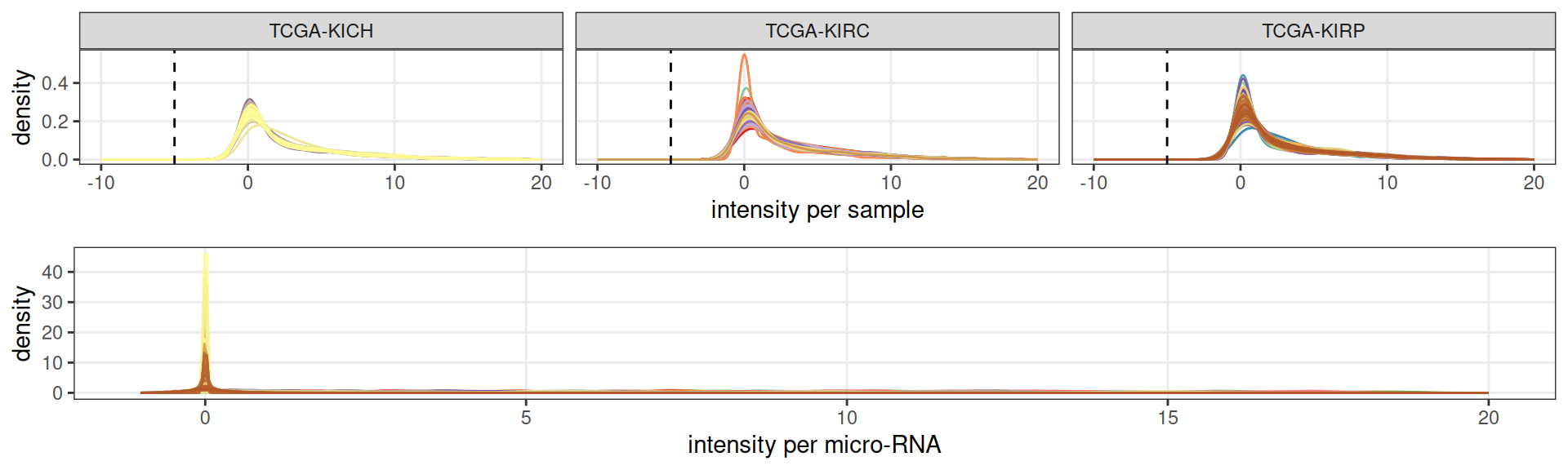
Let’s check the gene counts distributions across samples. We have counts information for 846 samples and a total of 743 micro-RNAs. There are no missing-values, so the count matrix has 100% occupancy. Looking at the counts distributions across the three kidney carcinomas, we observe an over-abundance of micro-RNAs with an average expression of 0 across the samples.
To best capture the biological signal, it would be beneficial to discard the micro-RNAs that have an expression of zero across all or most of the samples, so that we can focus on the ones that were expressed in the biopsies of the patients with kidney carcinomas.
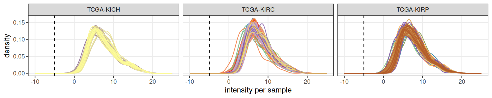
Filtering of lowly expressed micro-RNAs resulted in the exclusion of 553 of the 743 micro-RNAs.
In Figure 2 we can see the expression profiles across the kidney carcinomas samples of the 190 remaining micro-RNAs. Now, the average (log2) expression across samples is around 5.
4.3 Dimesionality Reduction and Dataset Exploration
4.3.1 Principal Component Analysis (PCA)
As we did for the transcriptomics data (see Chapter 2) and the proteomics one (see Chapter 3), the next step in the dataset exploration is to perform the Principal Component Analysis.
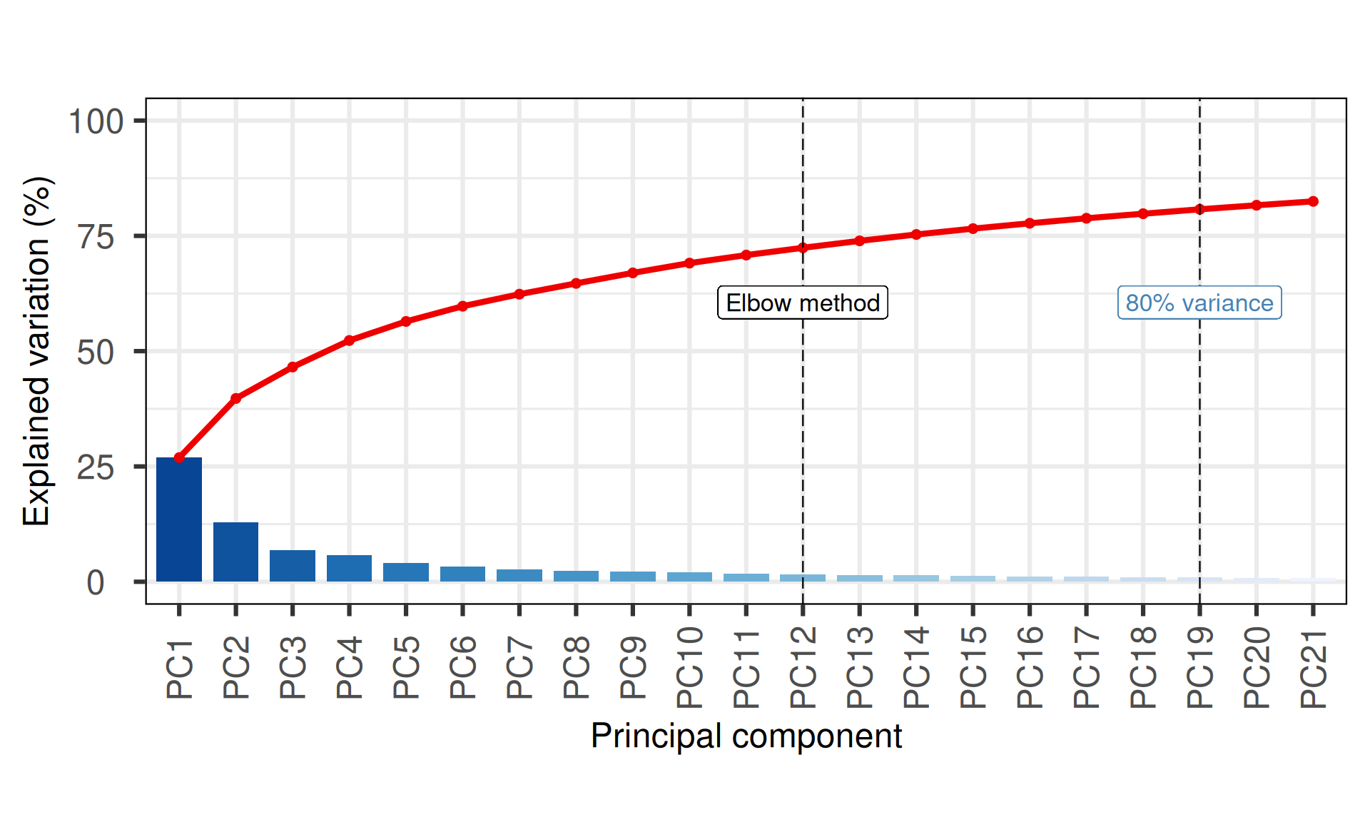
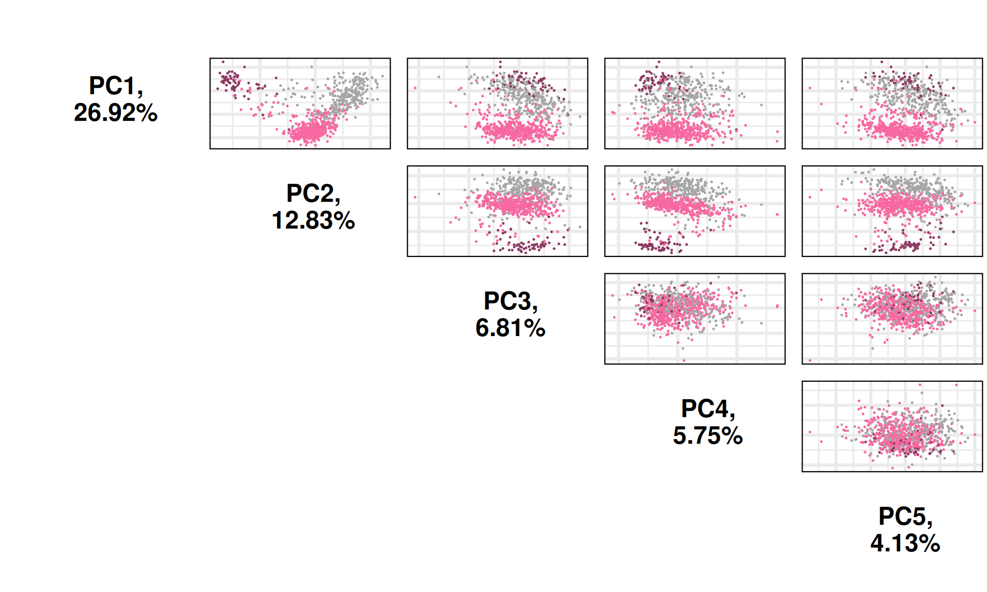
The first 19 Principal Components capture more than 80% of the variance in the Kidney cancers micro-RNAs datasets, with the first two components (PC1 and PC2) capturing almost 40% of the variance.
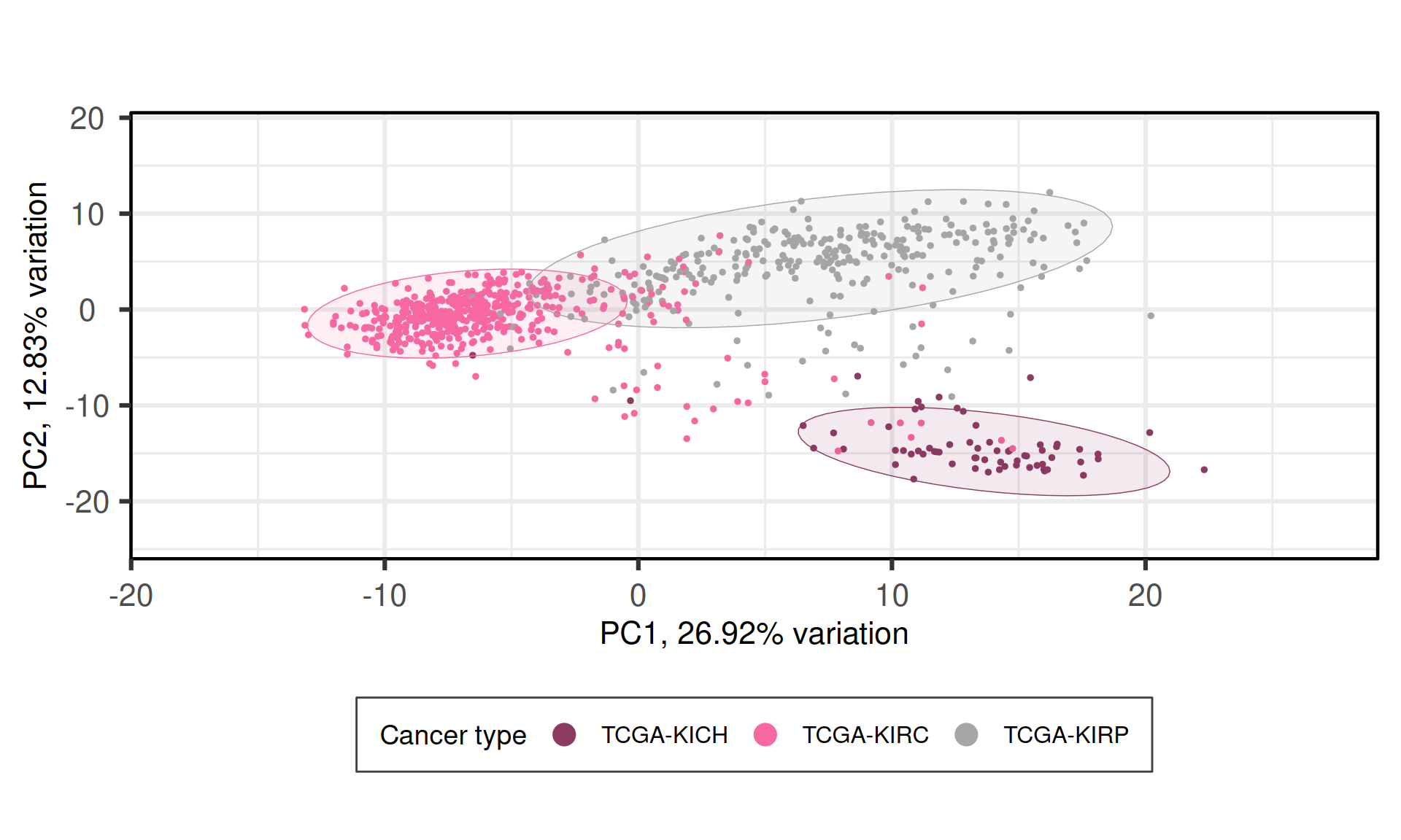
When we project the samples in the PC1 and PC2, we can see that the PC1 has a gradient of samples that go from KIRC to KIRP to KICH, which overlaps with the tail of KIRP samples. The second component PC2, instead, separated KIRC and KIRP from KICH. The first two principal components seems to separate the thee types of kidney carcinomas.
Let’s check the loadings (i.e.: 19 Principal Components capture more than 80% of the variance in the) for the top 4 Principal Components. These indicate which micro-RNAs are the more responsible to explain the position of the samples along the components, and the direction of this separation.
Looking at the top most variable genes, the following 8 micro-RNAs are the top loadings for the first 4 Principal Components:
- hsa-miR-10b-5p
- hsa-miR-126-3p
- hsa-miR-143-5p
- hsa-miR-144-5p
- hsa-miR-183-5p
- hsa-miR-200c-3p
- hsa-miR-204-5p
- hsa-miR-9-5p
Let’s now check the expression of the five top genes identified with the PCA across the cancer types:
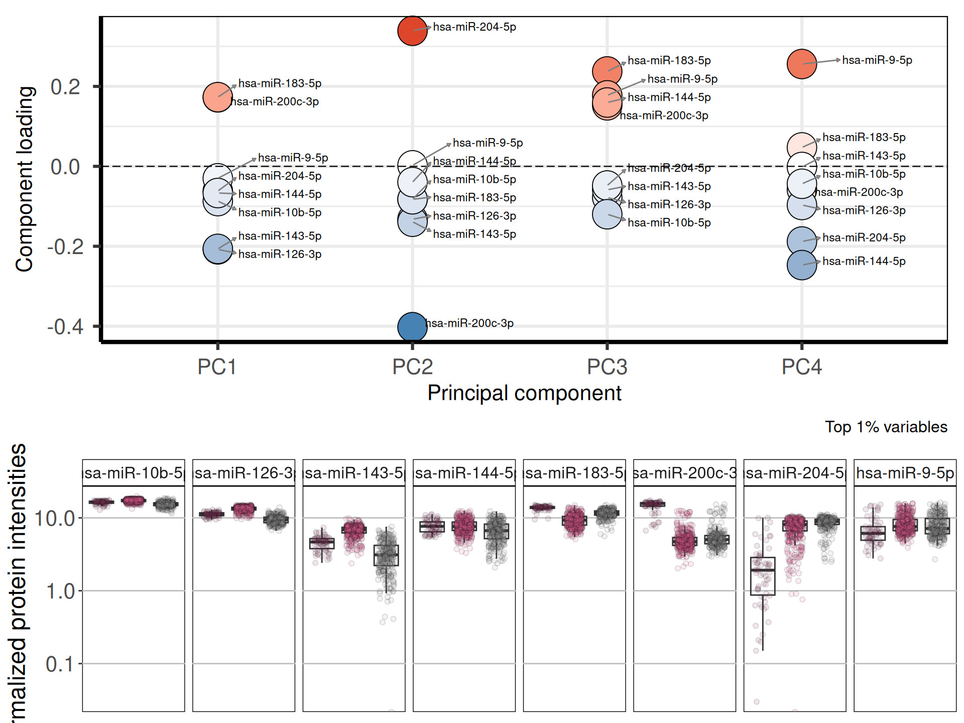
The miR-200 family is suggested to represent a good prognostic marker in clear cell renal cell carcinoma. In our analysis, hsa-miR-200c-3p seems to be overexpressed in KICH when compared to KIRC and KIRP. Lower expression of hsa-miR-200c-3p are associated with worse prognosis and carcinomas, in line with the better prognosis for KICH patients observed in our previous analysis (see Chapter 1).
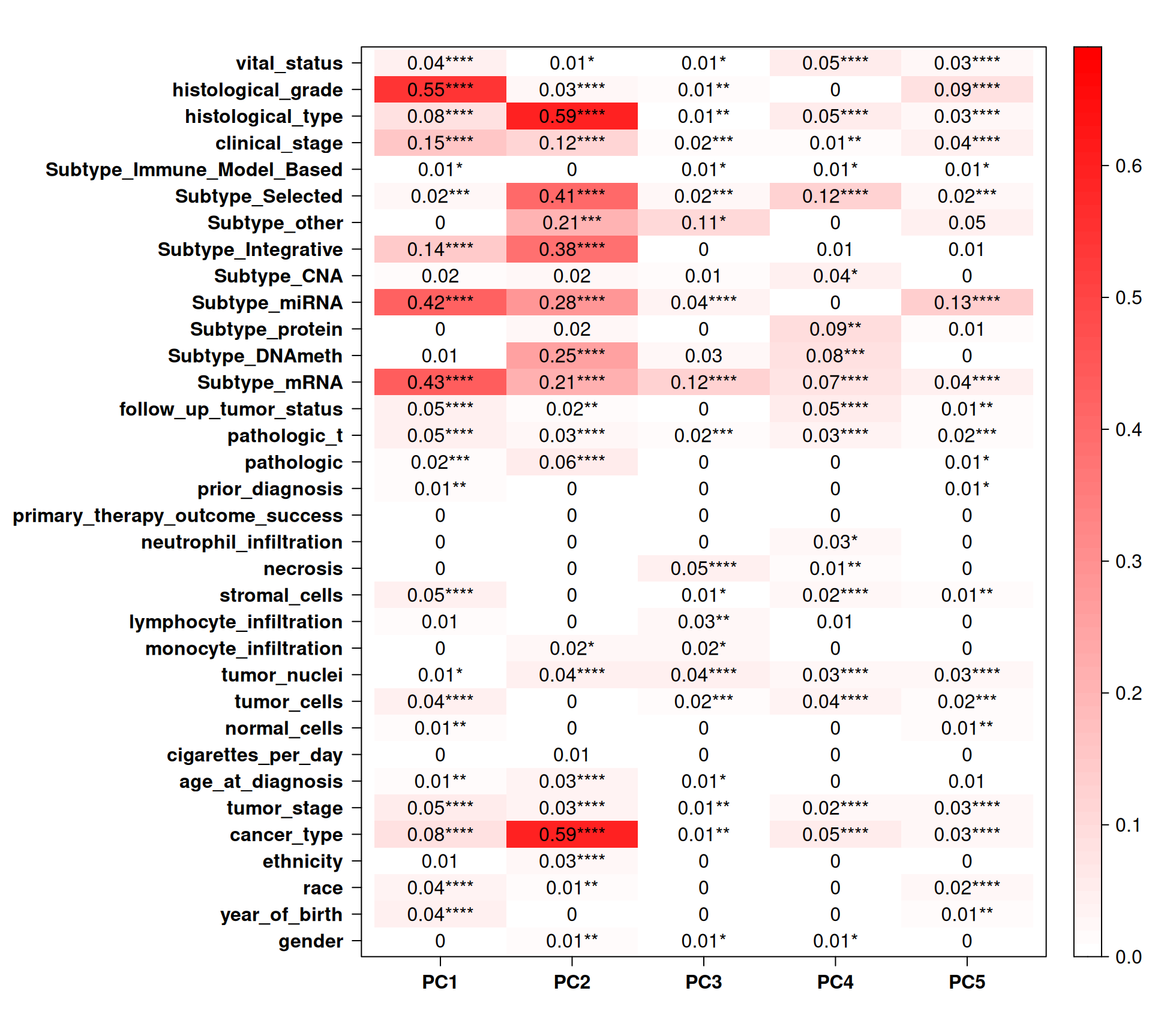
Let’s check the Pearson correlation with other clinical covariates.
Cancer type correlates with PC2, that, as we saw in the biplot in Figure 5, clearly separates KIRC and KIRP from KICH. Subtype miRNA and most of the other molecular subtypes assigned by TCGA strongly correlated with PC1 and PC2. Subtype miRNA also correlates with PC5. We observed little to no correlation with vital status or residual disease (follow up tumor status).
4.4 Differential gene expression analysis
In addition to cancer type, we saw that age, ethnicity (and race) and age had somewhat a correlation with the cancer types.
We may want to include this covariates in the differential gene expression analysis in order to include their contribution into the model.
4.4.1 Identification of differentially expressed micro-RNAs
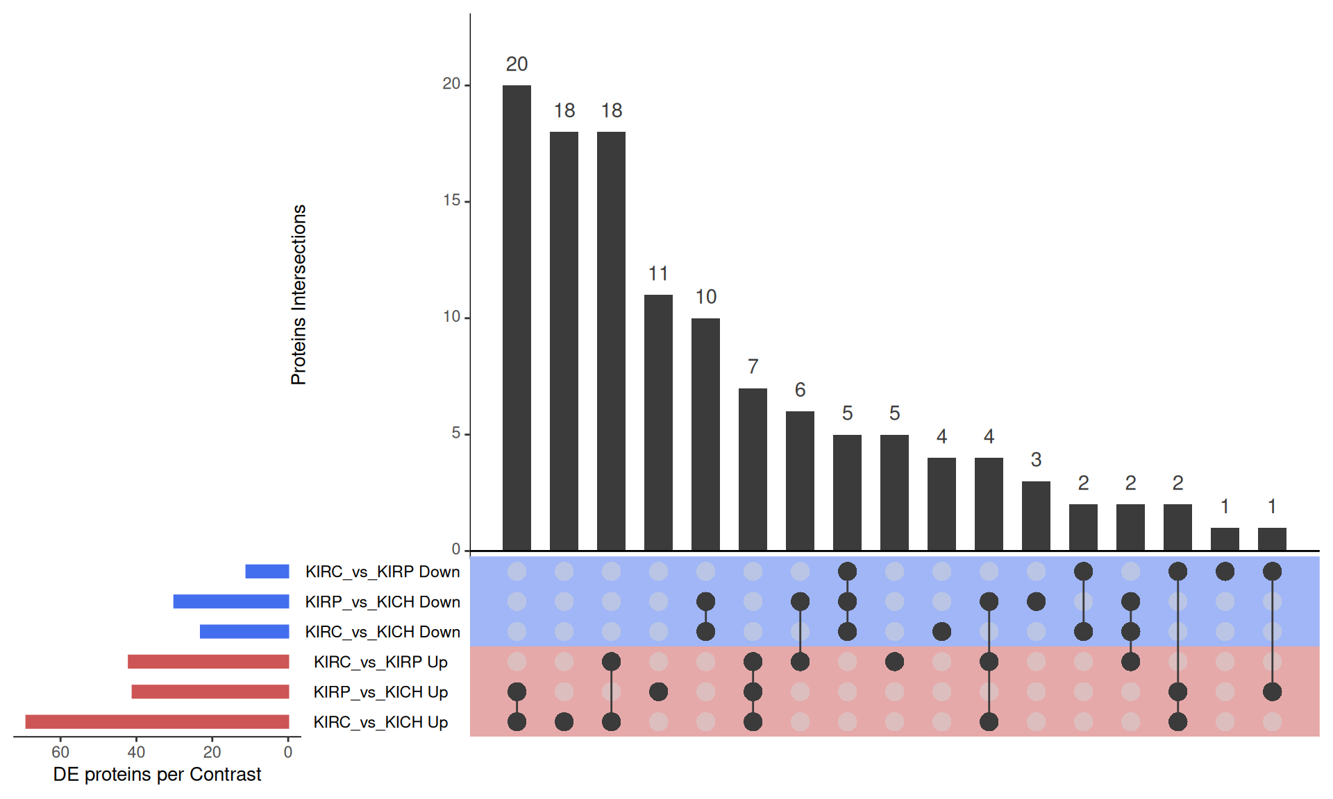
For micro-RNAs analyses, we use two arbitrary thresholds to retain genes that are significantly differentially expressed across the each comparison: an absolute logFold-Change (logFC) higher than 1, and an adjusted p-value lower than 0.05. This results in:
- KIRC_vs_KICH, 157 differentially expressed micro-RNAs, 118 upregulated and 49 downregulated
- KIRP_vs_KICH, 155 differentially expressed micro-RNAs, 87 upregulated and 68 downregulated
- KIRC_vs_KIRP, 163 differentially expressed micro-RNAs, 105 upregulated and 55 downregulated
As usual, we can visualize the logFC p-values relationships for all the micro-RNAs with a volcano plot.
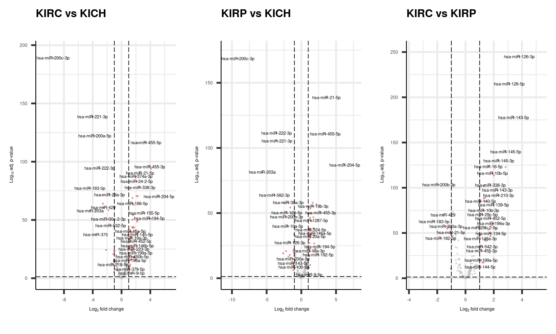
We can also check the logFC and adjusted p-value for the top 8 micro-RNAs that are the top loadings for the first 4 Principal Components and see how these micro-RNAs were differentially expressed across the comparisons.
We can confirm what we have naively observed at the level of micro-RNAs expression in Figure 7 while investigating the PCA loadings: hsa-miR-200c-3p and hsa-miR-204c-5p are the top loadings for PC2, which separates KIRC and KIRP from KICH, and indeed, these micro-RNAs are the most differentially expressed in the comparisons of KIRC and KIRP versus KICH, with hsa-miR-200c-3p strongly upregulated in KICH (> 9 fold difference), while hsa-miR-204c-5p is strongly downregulates in KICH (>5 fold difference).
The UpSet plot shows that KICH has a strong signature of 30 micro-RNAs that are differentially abundant when compared to KIRC or KIRP, including hsa-miR-34a-5p, hsa-miR-146a-5p, hsa-miR-146b-5p, hsa-miR-181a-3p, hsa-miR-204-5p and hsa-miR-200c-3p. KIRC, instead, has a signature of 20 micro-RNAs, including hsa-miR-155-5p.
Tables of differentially expressed micro-RNAs
4.5 Lessons Learnt
Based on micro-RNAs data, we have learnt:
- Exploratory analysis suggests:
- PC2 (12.83% variance) separates the three kidney carcinomas types.
- Differential Gene Expression analysis:
- here KIRC and KIRP seems more similar to each other (30 DGE microRNAs in common vs KICH).
- KIRC have 20 dysregulated miRNAs when compared to KIRP and KICH (including hsa-miR-155-5p)
- hsa-miR-155-5p (among the others) may contribute to regulate the metabolic reprogramming in KIRC by promoting glycolysis via PKM2, LDHA/LDHB, and GAPDH.
4.6 Session Information
Note
R version 4.3.3 (2024-02-29)
Platform: x86_64-pc-linux-gnu (64-bit)
Running under: Ubuntu 24.04.3 LTS

Matrix products: default
BLAS:   /usr/lib/x86_64-linux-gnu/blas/libblas.so.3.12.0
LAPACK: /usr/lib/x86_64-linux-gnu/lapack/liblapack.so.3.12.0

locale:
 [1] LC_CTYPE=en_US.UTF-8    LC_NUMERIC=C            LC_TIME=C
 [4] LC_COLLATE=en_US.UTF-8  LC_MONETARY=C           LC_MESSAGES=en_US.UTF-8
 [7] LC_PAPER=C              LC_NAME=C               LC_ADDRESS=C
[10] LC_TELEPHONE=C          LC_MEASUREMENT=C        LC_IDENTIFICATION=C

time zone: Europe/Brussels
tzcode source: system (glibc)

attached base packages:
[1] grid      stats4    stats     graphics  grDevices utils     datasets
[8] methods   base

other attached packages:
 [1] UpSetR_1.4.0           umap_0.2.10.0          stringr_1.5.1
 [4] scales_1.4.0           RColorBrewer_1.1-3     PCAtools_2.14.0
 [7] matrixStats_1.5.0      org.Hs.eg.db_3.18.0    gridExtra_2.3
[10] forcats_1.0.0          EnhancedVolcano_1.20.0 ggrepel_0.9.6
[13] ggplot2_3.5.2          edgeR_4.0.16           limma_3.58.1
[16] DT_0.33                dplyr_1.1.4            DOSE_3.28.2
[19] data.table_1.17.8      cowplot_1.2.0          clusterProfiler_4.10.1
[22] BiocSingular_1.18.0    BiocParallel_1.36.0    AnnotationDbi_1.64.1
[25] IRanges_2.36.0         S4Vectors_0.40.2       Biobase_2.62.0
[28] BiocGenerics_0.48.1

loaded via a namespace (and not attached):
  [1] jsonlite_2.0.0            magrittr_2.0.3
  [3] farver_2.1.2              rmarkdown_2.29
  [5] fs_1.6.6                  zlibbioc_1.48.2
  [7] vctrs_0.6.5               DelayedMatrixStats_1.24.0
  [9] memoise_2.0.1             RCurl_1.98-1.17
 [11] askpass_1.2.1             ggtree_3.10.1
 [13] htmltools_0.5.8.1         S4Arrays_1.2.1
 [15] SparseArray_1.2.4         gridGraphics_0.5-1
 [17] sass_0.4.10               bslib_0.9.0
 [19] htmlwidgets_1.6.4         plyr_1.8.9
 [21] cachem_1.1.0              igraph_2.1.4
 [23] lifecycle_1.0.4           pkgconfig_2.0.3
 [25] rsvd_1.0.5                Matrix_1.6-5
 [27] R6_2.6.1                  fastmap_1.2.0
 [29] gson_0.1.0                GenomeInfoDbData_1.2.11
 [31] MatrixGenerics_1.14.0     digest_0.6.37
 [33] aplot_0.2.8               enrichplot_1.22.0
 [35] patchwork_1.3.1           RSpectra_0.16-2
 [37] dqrng_0.4.1               irlba_2.3.5.1
 [39] crosstalk_1.2.1           RSQLite_2.4.2
 [41] beachmat_2.18.1           labeling_0.4.3
 [43] httr_1.4.7                polyclip_1.10-7
 [45] abind_1.4-8               compiler_4.3.3
 [47] bit64_4.6.0-1             withr_3.0.2
 [49] S7_0.2.0                  viridis_0.6.5
 [51] DBI_1.2.3                 ggforce_0.5.0
 [53] MASS_7.3-60.0.1           openssl_2.3.3
 [55] DelayedArray_0.28.0       HDO.db_0.99.1
 [57] tools_4.3.3               ape_5.8-1
 [59] scatterpie_0.2.5          glue_1.8.0
 [61] nlme_3.1-164              GOSemSim_2.28.1
 [63] shadowtext_0.1.5          reshape2_1.4.4
 [65] fgsea_1.35.6              generics_0.1.4
 [67] gtable_0.3.6              tidyr_1.3.1
 [69] tidygraph_1.3.1           ScaledMatrix_1.10.0
 [71] XVector_0.42.0            pillar_1.11.0
 [73] yulab.utils_0.2.0         splines_4.3.3
 [75] tweenr_2.0.3              treeio_1.26.0
 [77] lattice_0.22-5            bit_4.6.0
 [79] tidyselect_1.2.1          locfit_1.5-9.12
 [81] GO.db_3.18.0              Biostrings_2.70.3
 [83] knitr_1.50                xfun_0.52
 [85] graphlayouts_1.2.2        statmod_1.5.0
 [87] stringi_1.8.7             lazyeval_0.2.2
 [89] ggfun_0.2.0               yaml_2.3.10
 [91] evaluate_1.0.4            codetools_0.2-19
 [93] ggraph_2.2.1              tibble_3.3.0
 [95] qvalue_2.34.0             ggplotify_0.1.2
 [97] cli_3.6.5                 reticulate_1.43.0
 [99] jquerylib_0.1.4           dichromat_2.0-0.1
[101] Rcpp_1.1.0                GenomeInfoDb_1.38.8
[103] png_0.1-8                 parallel_4.3.3
[105] blob_1.2.4                sparseMatrixStats_1.14.0
[107] bitops_1.0-9              viridisLite_0.4.2
[109] tidytree_0.4.6            purrr_1.1.0
[111] crayon_1.5.3              rlang_1.1.6
[113] fastmatch_1.1-6           KEGGREST_1.42.0