4 Copy Number Variants
4.1 On this page
Biological insights and take-home messages are at the bottom of the page at section Lesson Learnt: Section 6.5.
- Here
4.2 Call the CNVs
To detect Copy Number Variants (CNVs) and major aneuploidies, we use the CNVnator pipeline. We use the bam files containing informations on aligned reads to the reference S288C genome, and we call CNVs based on changes of depth of mapped reads. The protocol we follow is:
- For each sample, run CNVnator for 500 bp and 1,000 bp bins;
- Retain only CNVs that are concordant for both bins;
- Identify common CNVs pattern;
- Identify genes affected by CNVs;
- GO, KEGG and Reactome pathways enrichment
First, we call CNVs with CNVnator, using 500 bp and 1,000 bp bins. Then, for each samples, we retain only CNVs that have been called with both bins, and that had a p-value < 0.05.
# prepare reference genome
while read line; do
  if [[ ${line:0:1} == '>' ]]; then
    outfile=${line#>}.fa;
    echo $line > $outfile;
  else
    echo $line >> $outfile;
  fi;
done < Saccharomyces_RefGen.fa

#run CNVnator from the docker image
chmod 777 09_CNVs/

for file in *.bam; do

  NAME=$(basename $file .S288C.align.sort.md.r.bam);

  docker run -v /home/andrea/03_KVEIK/09_CNVs/:/data wwliao/cnvnator
    cnvnator \
    -root ./out."${NAME}".root \
    -genome
    ./00_refgen/Saccharomyces_cerevisiae.EF4.73.dna.chromosome.all.fa \
    -tree $file;

  for BIN in 500 1000; do

    docker run -v /home/andrea/03_KVEIK/09_CNVs/:/data wwliao/cnvnator
      cnvnator \
      -root ./out."${NAME}".root \
      -genome
      ./00_refgen/Saccharomyces_cerevisiae.EF4.73.dna.chromosome.all.fa \
      -his $BIN -d ./;

    docker run -v /home/andrea/03_KVEIK/09_CNVs/:/data wwliao/cnvnator
      cnvnator \
      -root ./out."${NAME}".root \
      -stat $BIN;

    docker run -v /home/andrea/03_KVEIK/09_CNVs/:/data wwliao/cnvnator
      cnvnator \
      -ngc \
      -root ./out."${NAME}".root \
      -partition $BIN;

    docker run -v /home/andrea/03_KVEIK/09_CNVs/:/data wwliao/cnvnator
      cnvnator \
      -ngc \
      -root ./out."${NAME}".root \
      -call $BIN > "${NAME}".CNV_"${BIN}"bin.tab;

  done;
done

chmod 755 09_CNVs/
# Filter CNVs and merge 500bp 1000bp windows
while read line; do

  python3.5 ~/CNVnator_merger.py \
    --input_1 $line.CNV_500bin.tab \
    --input_2 $line.CNV_1000bin.tab \
    --sample $line > $line.CNVmerged.500-1000.tab;

done < ../sample.lst

cat *merged.500-1000.tab > Vikings.CNVsmerged.all.tab
Then we plot the CNV that we have identified. To facilitate the visualization, duplications have been amplified up to 10X, while deletion have been reduced to 1X. Farmhouse yeasts have been clustered based on their geographical origin, in order from the top to the bottom:
- North-West Norway;
- South-West Norway;
- Central-Eastern Norway;
- Latvia;
- Lithuania;
- Russia.
# upload files
V_CNVs_1000 = read.delim("data/p01-04/Vikings.CNVsmerged.all.mod.tab", header = TRUE)

# reformat data
V_CNVs_1000$chr = factor(V_CNVs_1000$chr, levels = c("I", "II", "III", "IV", "V", "VI",
                                                     "VII", "VIII", "IX", "X", "XI", "XII",
                                                     "XIII", "XIV", "XV", "XVI"))

# group kveiks by geographical origin
V_CNVs_1000$strain = factor(V_CNVs_1000$strain, levels = c(
  "41R10", "21R38", "9R40", "17P5", "SortdalEbbe1", "3R11", "21P1", "41R15", "Hornindal1", "Hornindal2", "1R16", "2R23", "8R19", "Muri",
   "k7R25", "38R16", "44R32", "19R18", "44R7", "6R15", "Laerdal2", "7R7", "14R6", "14R30",
   "27R17", "28P1", "28P6", "28R21", "28R33", "28R8",
   "42R20", "42R31", "45P5", "45R11",
   "46R12", "46R37", "16R23", "16R37",
   "39R20", "40R14", "40R1", "40R20",
   "Granvin1", "Voss1"
))

# plot
p = ggplot(V_CNVs_1000) +
  geom_rect(aes(xmin = start, xmax = stop, ymin = start_y, ymax = stop_y, fill = CNV), color="black", size = 0.001) +
  scale_fill_gradient2(midpoint = 0, low = "#84ceff", mid = "white", high = "#ffb584",
                       limits = c(0.1, 10), na.value = "grey75", trans = "log") +
  facet_grid(strain~chr, scales = "free", space = "free_x") +
  labs(title = "CNVs Distribution: 500-1,000 bp bin",
       fill = "log10 ReadDepth") +
  theme(plot.title = element_text(size = 28, hjust = 0.5),
        axis.ticks = element_blank(),
        axis.title = element_blank(),
        axis.text.x = element_blank(),
        axis.text.y = element_blank(),
        legend.position = "none",
        panel.background = element_blank(),
        panel.spacing.x = unit(0.05, "lines"),
        panel.spacing.y = unit(0.05, "lines"),
        panel.border = element_rect(colour = "black", fill = NA),
        strip.background = element_rect(colour = "black", fill = "grey90"),
        strip.text.x = element_text(size = 10),
        strip.text.y = element_text(size = 14, angle = 0))

# change facet colors
g = ggplot_gtable(ggplot_build(p))
stripr = which(grepl("strip-r", g$layout$name))
fills = c("#0571B0", "#0571B0", "#0571B0", "#0571B0", "#0571B0", "#0571B0", "#0571B0", "#0571B0",
          "#0571B0", "#0571B0", "#0571B0", "#0571B0", "#0571B0", "#0571B0", "#92C5DE", "#92C5DE",
          "#92C5DE", "#92C5DE", "#92C5DE", "#92C5DE", "#92C5DE", "#92C5DE", "#92C5DE", "#92C5DE",
          "#008470", "#008470", "#008470", "#008470", "#008470", "#008470", "#FFDA00", "#FFDA00",
          "#FFDA00", "#FFDA00", "#FBA01D", "#FBA01D", "#FBA01D", "#FBA01D", "#A6611A", "#A6611A",
          "#A6611A", "#A6611A", "grey75", "grey75")
k = 1
for (i in stripr) {
  j = which(grepl("rect", g$grobs[[i]]$grobs[[1]]$childrenOrder))
  g$grobs[[i]]$grobs[[1]]$children[[j]]$gp$fill = fills[k]
  k = k + 1
}
grid::grid.draw(g)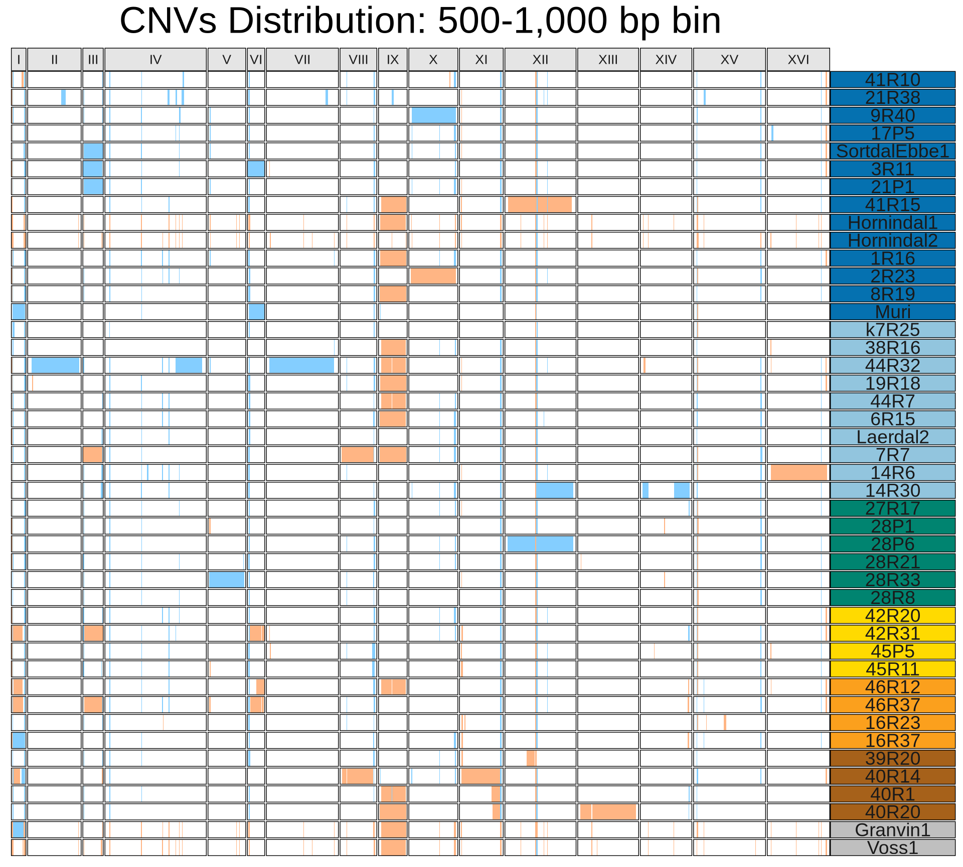
While there is no clear signature associated with kveiks geographic origin, it looks like there are common CNVs shared between farmhouse yeasts that are instead absent in industrial yeasts. Let’s clearly identify them.
There are the apparent trends:
- 5 out of 69 CNVs are shared among all Kveiks
- Granvin1, Hornindal1, Hornindal2, Voss1 have similar CNV fingerprint
4.3 Identify common CNVs in Farmhouse yeasts
We have a bunch of CNVs called on 44 different kveiks Some CNVs that are called on the same position on multiple samples, maybe differs for few hundred base pairs. To identify the “average” conserved CNV, we use a custom python script that collapse this windows, a sort of ad hoc bedtools merge for CNVs positions.
# generate overlapping windows
for i in "\tI\t" "\tII\t" "\tIII\t" "\tIV\t" "\tV\t" "\tVI\t" "\tVII\t" \
  "\tVIII\t" "\tIX\t" "\tX\t" "\tXI\t" "\tXII\t" "\tXIII\t" "\tXIV\t" \
  "\tXV\t" "\tXVI\t" "\tMito\t"; do
  grep -P "${i}" Vikings.CNVsmerged.all.tab \
    | cut -f 2-4 \
    | sort -u \
    | sort -k2,2n;
done > temp.bed;
bedtools merge -i temp.bed > Vikings.CNVsmerged.all.bed;
rm temp.bed;

python3.8 Vikings.overlapCNVs.py \
  --allCNVs Vikings.CNVsmerged.all.tab \
  --bed Vikings.CNVsmerged.all.bed \
  > Vikings.CNVsmerged.all.matrix.tab
Let’s check the CNVs distributions:
Let’s select CNVs present in at least 90% (N=40) of the sequenced farmhouse yeasts, and plot them. I would like to add as well the 4 large genomics variants in chromosomes I, III, VI and IX.
There are 11 CNVs shared between 40 farmhouse yeasts or more.
# create CNV matrix for the heatmap
matrix_heat = as.matrix(matrix.d75[, c(4:ncol(matrix.d75))])
matrix_heat = ifelse(matrix_heat < 1, -1,
                     ifelse(matrix_heat > 1, 1, matrix_heat))
rownames(matrix_heat) = paste(paste(matrix.d75[, 1], matrix.d75[, 2], sep = ":"), matrix.d75[, 3], sep = "-")

# create annotations
kveiks_geo = data.frame(
  c("41R10", "21R38", "9R40", "17P5", "SortdalEbbe1", "3R11", "21P1", "41R15", "Hornindal1", "Hornindal2", "1R16", "2R23", "8R19", "Muri",
    "k7R25", "38R16", "44R32", "19R18", "44R7", "6R15", "Laerdal2", "7R7", "14R6", "14R30",
    "27R17", "28P1", "28P6", "28R21", "28R33", "28R8",
    "42R20", "42R31", "45P5", "45R11",
    "46R12", "46R37", "16R23", "16R37",
    "39R20", "40R14", "40R1", "40R20",
    "Granvin1", "Voss1"),
  c("North-West Norway", "North-West Norway", "North-West Norway", "North-West Norway", "North-West Norway", "North-West Norway", "North-West Norway", "North-West Norway", "North-West Norway", "North-West Norway", "North-West Norway", "North-West Norway", "North-West Norway", "North-West Norway",
    "South-West Norway", "South-West Norway", "South-West Norway", "South-West Norway", "South-West Norway", "South-West Norway", "South-West Norway", "South-West Norway", "South-West Norway", "South-West Norway",
    "Central-Eastern Norway", "Central-Eastern Norway", "Central-Eastern Norway", "Central-Eastern Norway", "Central-Eastern Norway", "Central-Eastern Norway",
    "Latvia", "Latvia", "Latvia", "Latvia",
    "Lithuania", "Lithuania", "Lithuania", "Lithuania",
    "Russia", "Russia", "Russia", "Russia",
    "Other", "Other"))
colnames(kveiks_geo) = c("kveik", "geo")
rownames(kveiks_geo) = kveiks_geo$kveik

ComplexHeatmap::Heatmap(
  matrix_heat,
  cluster_rows = FALSE,
  column_dend_reorder = TRUE,
  col = colorRamp2(c(-1, 0, 1), rev(brewer.pal(n = 3, name = "RdBu"))),
  na_col = "grey75",
  top_annotation = HeatmapAnnotation(
    Geographic_origin = as.matrix(kveiks_geo$geo),
    col = list(Geographic_origin = c("North-West Norway" = "#0571B0",
                                     "South-West Norway" = "#92C5DE",
                                     "Central-Eastern Norway" = "#008470",
                                     "Latvia" = "#FFDA00",
                                     "Lithuania" = "#FBA01D",
                                     "Russia" = "#A6611A",
                                     "Other" = "grey50"))
  ),
  show_row_names = TRUE,
  show_column_names = TRUE,
  show_row_dend = FALSE,
  show_heatmap_legend = FALSE,
  row_title = "CNVs",
  column_title_side = "bottom"
)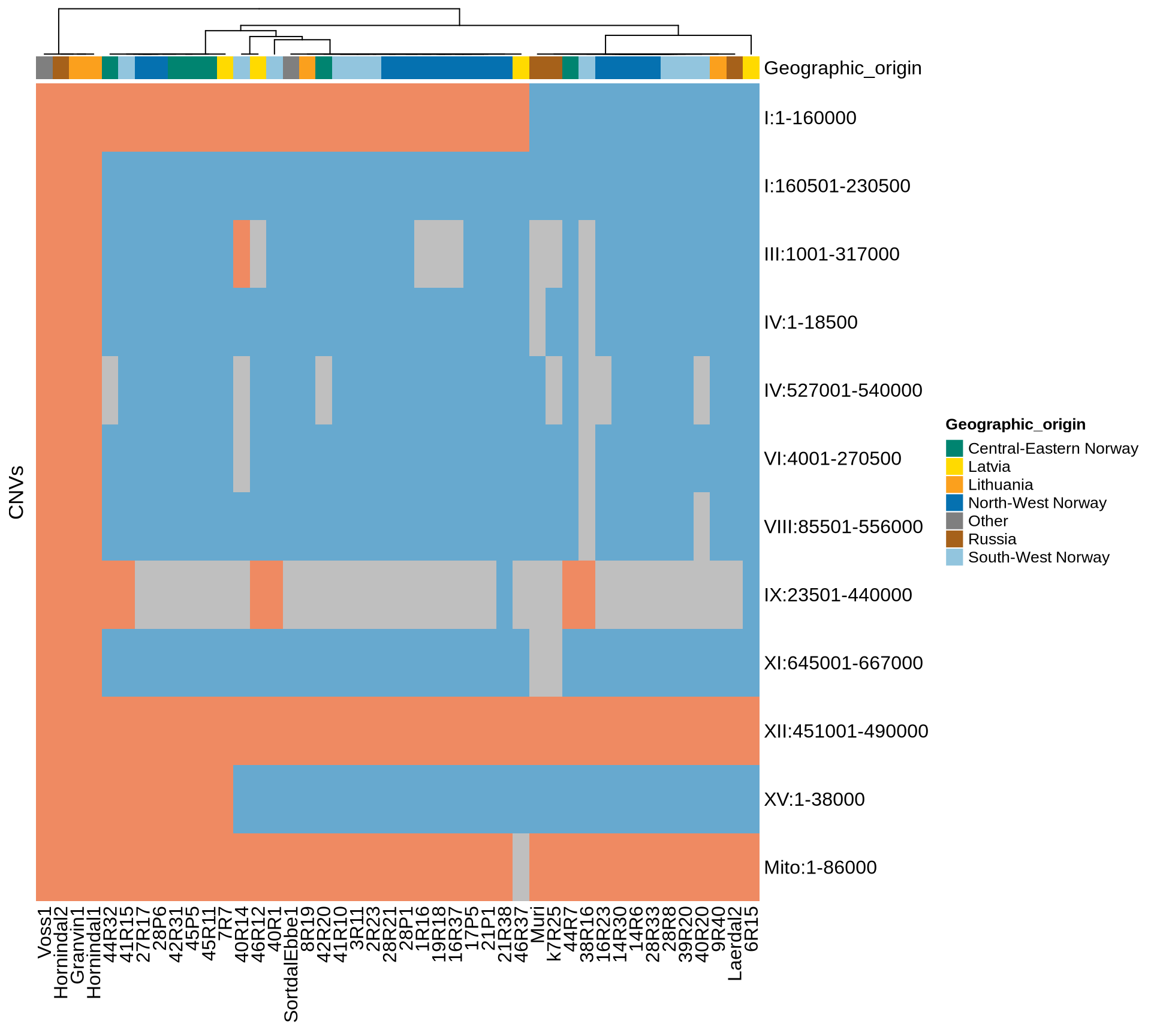
There are 69 high confidence CNVs, of which 5 (4 deletions and 1 duplication) of them are shared among all Kveiks. Interestingly, the two deletions in chromosome I and the one in chromosome XV are duplications in the lineage “Granvin1, Hornindal1, Hornindal2, Voss1”. Granvin1, Hornindal1, Hornindal2, Voss1 shares a unique fingerprint of 39 conserved CNVs scattered across 15 chromosomes.
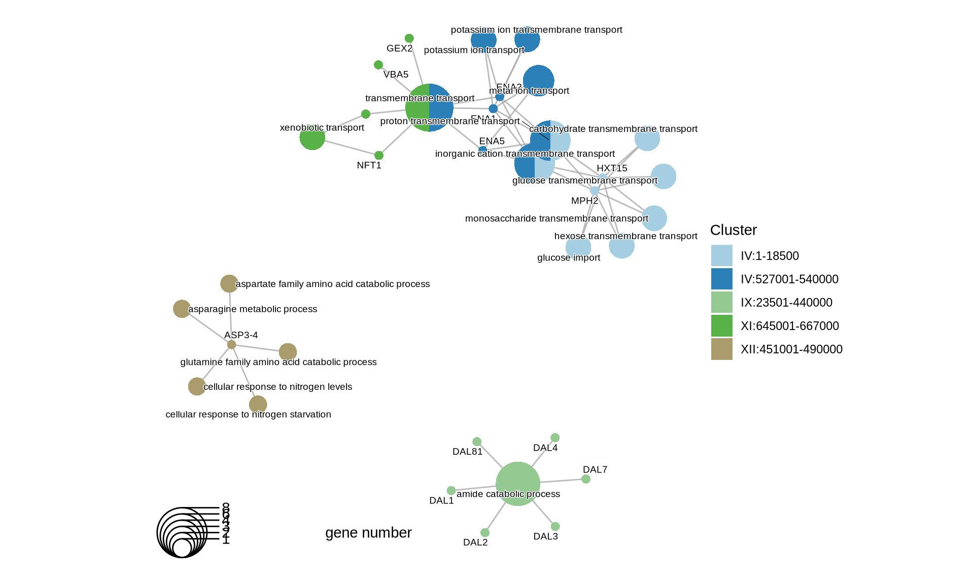
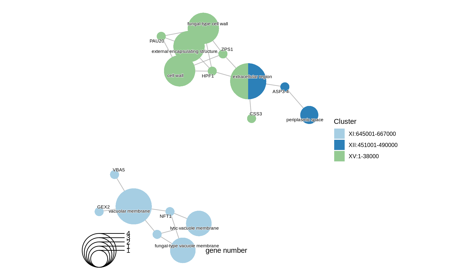
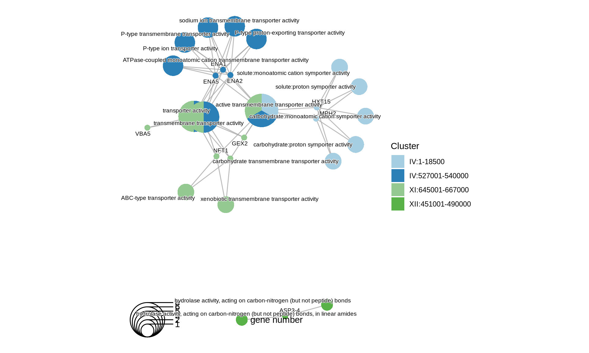
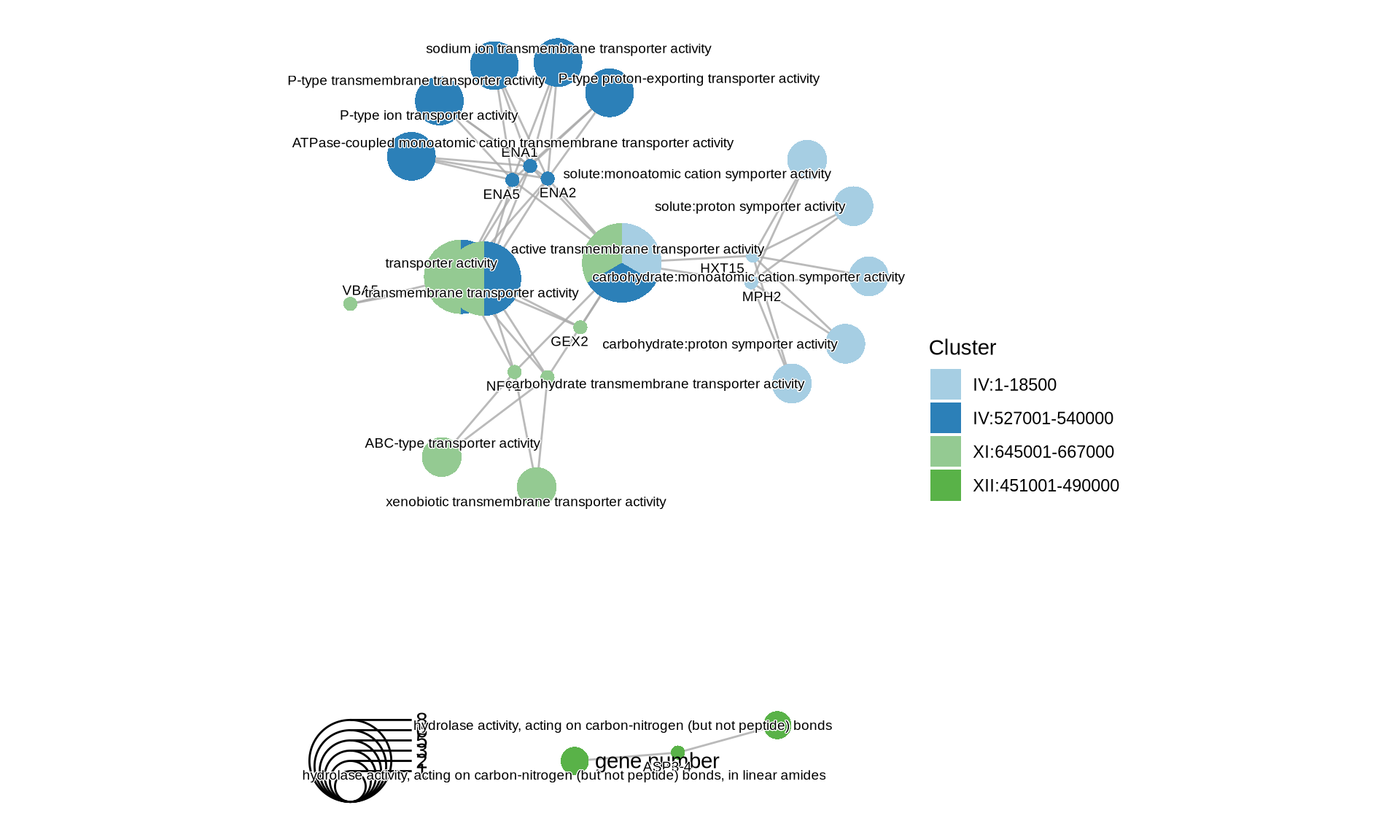
4.4 CNV Functional Enrichment
Let’s see which genes (and corresponding functions) are interested by the CNVs that we identify in the farmhouse yeasts. We will run the following functional analyses:
- over-represented GO terms;
- enriched GO terms;
- over-represented KEGG pathways;
- enriched KEGG pathways;
- over-represented Reactome pathways;
- enriched Reactome pathwyas.
# retrieve S. cerevisiae genome annotation
Scere_DB = biomaRt::useMart(
  biomart = "ENSEMBL_MART_ENSEMBL",
  dataset = "scerevisiae_gene_ensembl"
)
Scere_DB_table = biomaRt::getBM(
  attributes = c(
    "ensembl_gene_id",
    "ensembl_peptide_id",
    "external_gene_name",
    "entrezgene_id",
    "description",
    "chromosome_name",
    "start_position",
    "end_position"
  ),
  mart = Scere_DB
)

# build list of reference databases used for annotation steps
ref_DB_list = c("org.Sc.sgd.db", "yeast", "scerevisiae")

# create yeasts GO terms universe
GO_universe = data.frame(matrix(nrow = nrow(Scere_DB_table), ncol = 2))
names(GO_universe) = c("ENSEMBL", "EntrezID")
GO_universe$ENSEMBL = Scere_DB_table$ensembl_gene_id
# populate GO universe
for(k in 1:nrow(GO_universe)){
  # force to get only the first term if multiple are retrieved (sic!)
  ENSEMBL = GO_universe[k, 1]
  GO_universe[k, 2] = tryCatch(
    Scere_DB_table[which(Scere_DB_table[, 1] == ENSEMBL),  c(4)][[1]],
    error = function(e) { NA }
  )
}
GO_universe = as.character(c(GO_universe[!is.na(GO_universe$EntrezID), ]$EntrezID))

# drop mitochondria
matrix_heat = matrix_heat[-which(rownames(matrix_heat) == "Mito:1-86000"), ]

# retrieve genes by CNV
CNV_genes_DB = list()
for(i in 1:nrow(matrix_heat)){

  # get CNVs cohordinates
  chromosome = stringr::str_split(rownames(matrix_heat)[i], ":")[[1]][1]
  positions = stringr::str_split(rownames(matrix_heat)[i], ":")[[1]][2]
  start_position = stringr::str_split(positions, "-")[[1]][1]
  end_position = stringr::str_split(positions, "-")[[1]][2]

  # get genes in CNV
  CNV_genes_DB[[rownames(matrix_heat)[i]]] = biomaRt::getBM(
    attributes = c(
      "ensembl_gene_id",
      "ensembl_peptide_id",
      "external_gene_name",
      "entrezgene_id",
      "description",
      "chromosome_name",
      "start_position",
      "end_position"
    ),
    filters = c("chromosome_name", "start", "end"),
    values = list(chromosome = chromosome,
                  start = start_position,
                  end = end_position),
    mart = Scere_DB
  )

}

# retrieve genes
gene_cluster = list()
for(i in 1:length(CNV_genes_DB)){
  gene_cluster[[names(CNV_genes_DB)[[i]]]] = as.character(CNV_genes_DB[[i]]$entrezgene_id[!is.na(CNV_genes_DB[[i]]$entrezgene_id)])
}
Let’s compare all enrichment together
Usually I would convert the names in the enriched cluster with the DOSE package, with something like: DOSE::setReadable(BP, OrgDb = org.Sc.sgd.db, keyType = "ENTREZID"), however, org.Sc.sgd.db does not encode the gene names as SYMBOL like it happens in other reference genomes from ENSEMBL (org.Sc.sgd.db is maintained by SGD).
Therefore I need a less elegant workaround to manually replace the ENTREZID with the corresponding gene symbols to make the enrichment comparisons more interepretable.
# enrich
BP = compareCluster(
  geneCluster = gene_cluster,
  fun = "enrichGO",
  pvalueCutoff = 0.05,
  OrgDb = ref_DB_list[[1]],
  ont = "BP"
)

# map gene symbols
BP@keytype = "SYMBOL"
my_symbols = c()
for(k in 1:length(BP@geneClusters)){
  for(i in 1:length(BP@geneClusters[[k]])){
    ENTREZ = BP@geneClusters[[k]][[i]]
    SYMBOL = Scere_DB_table[which(Scere_DB_table$entrezgene_id == ENTREZ), ]$external_gene_name
    my_symbols[i] = SYMBOL
  }
  BP@geneClusters[[k]] = my_symbols
}
for(k in 1:length(BP@compareClusterResult$geneID)){
  my_vec = BP@compareClusterResult$geneID[[k]]
  my_vec = stringr::str_split(my_vec, "/")[[1]]
  for(i in 1:length(my_vec)){
    ENTREZ = my_vec[[i]]
    SYMBOL = Scere_DB_table[which(Scere_DB_table$entrezgene_id == ENTREZ), ]$external_gene_name
    my_vec[[i]] = SYMBOL[[1]]
  }
  my_vec = paste(my_vec, collapse = "/")
  BP@compareClusterResult$geneID[[k]] = my_vec
}

# plot
p1 = enrichplot::dotplot(BP, includeAll = TRUE) +
  scale_colour_gradientn(colours = rev(colorRampPalette(brewer.pal(7, "Reds"))(37))) +
  guides(colour = guide_colorbar(reverse = TRUE)) +
  theme(plot.title = element_text(size = 22, hjust = 0.5)) +
  theme(axis.text.x=element_text(angle = 45, hjust = 1))

p2 = cnetplot(BP) +
  scale_fill_manual(values = colorRampPalette(brewer.pal(10, "Paired"))(length(BP@geneClusters))) +
  theme(plot.title = element_text(size = 22, hjust = 0.5))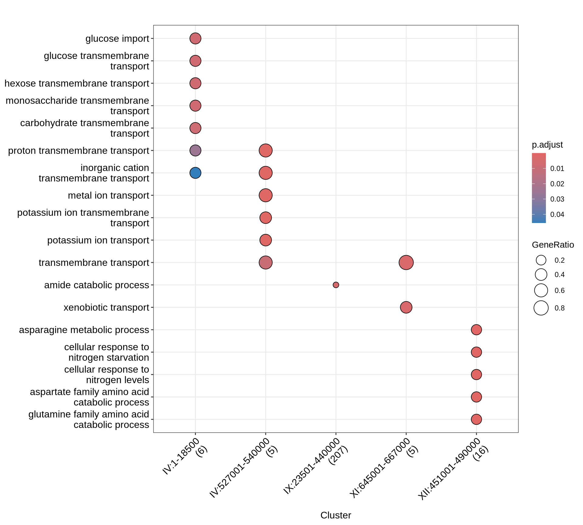
# enrich
CC = compareCluster(
  geneCluster = gene_cluster,
  fun = "enrichGO",
  pvalueCutoff = 0.05,
  OrgDb = ref_DB_list[[1]],
  ont = "CC"
)

# map gene symbols
CC@keytype = "SYMBOL"
my_symbols = c()
for(k in 1:length(CC@geneClusters)){
  for(i in 1:length(CC@geneClusters[[k]])){
    ENTREZ = CC@geneClusters[[k]][[i]]
    SYMBOL = Scere_DB_table[which(Scere_DB_table$entrezgene_id == ENTREZ), ]$external_gene_name
    my_symbols[i] = SYMBOL
  }
  CC@geneClusters[[k]] = my_symbols
}
for(k in 1:length(CC@compareClusterResult$geneID)){
  my_vec = CC@compareClusterResult$geneID[[k]]
  my_vec = stringr::str_split(my_vec, "/")[[1]]
  for(i in 1:length(my_vec)){
    ENTREZ = my_vec[[i]]
    SYMBOL = Scere_DB_table[which(Scere_DB_table$entrezgene_id == ENTREZ), ]$external_gene_name
    my_vec[[i]] = SYMBOL[[1]]
  }
  my_vec = paste(my_vec, collapse = "/")
  CC@compareClusterResult$geneID[[k]] = my_vec
}

# plot
p1 = enrichplot::dotplot(CC, includeAll = TRUE) +
  scale_colour_gradientn(colours = rev(colorRampPalette(brewer.pal(7, "Reds"))(37))) +
  guides(colour = guide_colorbar(reverse = TRUE)) +
  theme(plot.title = element_text(size = 22, hjust = 0.5)) +
  theme(axis.text.x=element_text(angle = 45, hjust = 1))

p2 = cnetplot(CC) +
  scale_fill_manual(values = colorRampPalette(brewer.pal(10, "Paired"))(length(CC@geneClusters))) +
  theme(plot.title = element_text(size = 22, hjust = 0.5))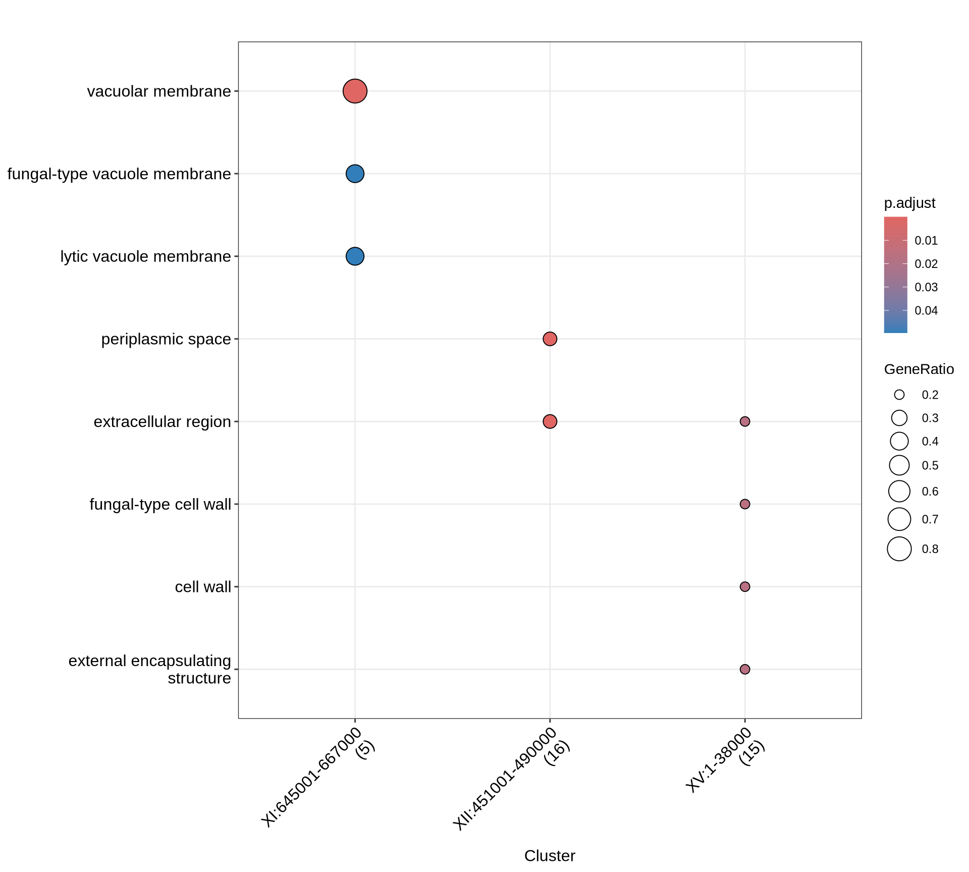
# enrich
MF = compareCluster(
  geneCluster = gene_cluster,
  fun = "enrichGO",
  pvalueCutoff = 0.05,
  OrgDb = ref_DB_list[[1]],
  ont = "MF"
)

# map gene symbols
MF@keytype = "SYMBOL"
my_symbols = c()
for(k in 1:length(MF@geneClusters)){
  for(i in 1:length(MF@geneClusters[[k]])){
    ENTREZ = MF@geneClusters[[k]][[i]]
    SYMBOL = Scere_DB_table[which(Scere_DB_table$entrezgene_id == ENTREZ), ]$external_gene_name
    my_symbols[i] = SYMBOL
  }
  MF@geneClusters[[k]] = my_symbols
}
for(k in 1:length(MF@compareClusterResult$geneID)){
  my_vec = MF@compareClusterResult$geneID[[k]]
  my_vec = stringr::str_split(my_vec, "/")[[1]]
  for(i in 1:length(my_vec)){
    ENTREZ = my_vec[[i]]
    SYMBOL = Scere_DB_table[which(Scere_DB_table$entrezgene_id == ENTREZ), ]$external_gene_name
    my_vec[[i]] = SYMBOL[[1]]
  }
  my_vec = paste(my_vec, collapse = "/")
  MF@compareClusterResult$geneID[[k]] = my_vec
}

# plot
p1 = enrichplot::dotplot(MF, includeAll = TRUE) +
  scale_colour_gradientn(colours = rev(colorRampPalette(brewer.pal(7, "Reds"))(37))) +
  guides(colour = guide_colorbar(reverse = TRUE)) +
  theme(plot.title = element_text(size = 22, hjust = 0.5)) +
  theme(axis.text.x=element_text(angle = 45, hjust = 1))

p2 = cnetplot(MF) +
  scale_fill_manual(values = colorRampPalette(brewer.pal(10, "Paired"))(length(MF@geneClusters))) +
  theme(plot.title = element_text(size = 22, hjust = 0.5))
# enrich
KEGG = compareCluster(
  geneCluster = gene_cluster,
  fun = "enrichKEGG",
  pvalueCutoff = 0.05,
  organism = "sce"
)

# map gene symbols
KEGG@keytype = "SYMBOL"
my_symbols = c()
for(k in 1:length(KEGG@geneClusters)){
  for(i in 1:length(KEGG@geneClusters[[k]])){
    ENTREZ = KEGG@geneClusters[[k]][[i]]
    SYMBOL = Scere_DB_table[which(Scere_DB_table$entrezgene_id == ENTREZ), ]$external_gene_name
    my_symbols[i] = SYMBOL
  }
  KEGG@geneClusters[[k]] = my_symbols
}
for(k in 1:length(KEGG@compareClusterResult$geneID)){
  my_vec = KEGG@compareClusterResult$geneID[[k]]
  my_vec = stringr::str_split(my_vec, "/")[[1]]
  for(i in 1:length(my_vec)){
    ENTREZ = my_vec[[i]]
    SYMBOL = Scere_DB_table[which(Scere_DB_table$entrezgene_id == ENTREZ), ]$external_gene_name
    my_vec[[i]] = SYMBOL[[1]]
  }
  my_vec = paste(my_vec, collapse = "/")
  KEGG@compareClusterResult$geneID[[k]] = my_vec
}

# plot
p1 = enrichplot::dotplot(KEGG, includeAll = TRUE) +
  scale_colour_gradientn(colours = rev(colorRampPalette(brewer.pal(7, "Reds"))(37))) +
  guides(colour = guide_colorbar(reverse = TRUE)) +
  theme(plot.title = element_text(size = 22, hjust = 0.5)) +
  theme(axis.text.x=element_text(angle = 45, hjust = 1))

p2 = cnetplot(KEGG) +
  scale_fill_manual(values = colorRampPalette(brewer.pal(10, "Paired"))(length(KEGG@geneClusters))) +
  theme(plot.title = element_text(size = 22, hjust = 0.5))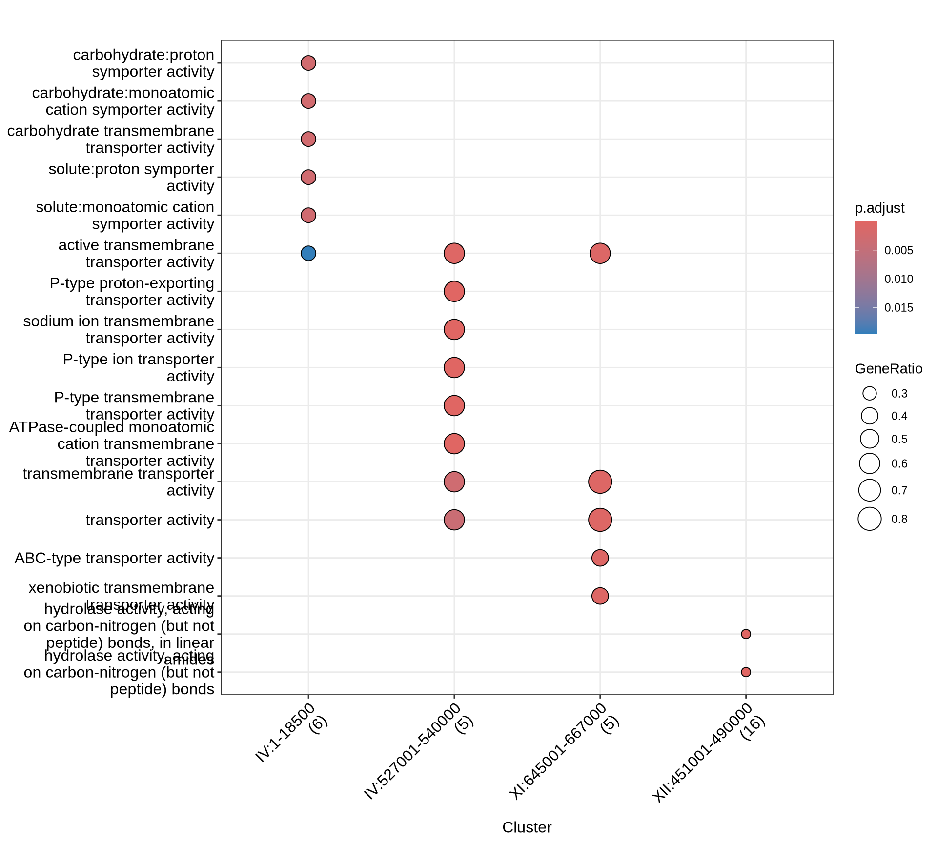
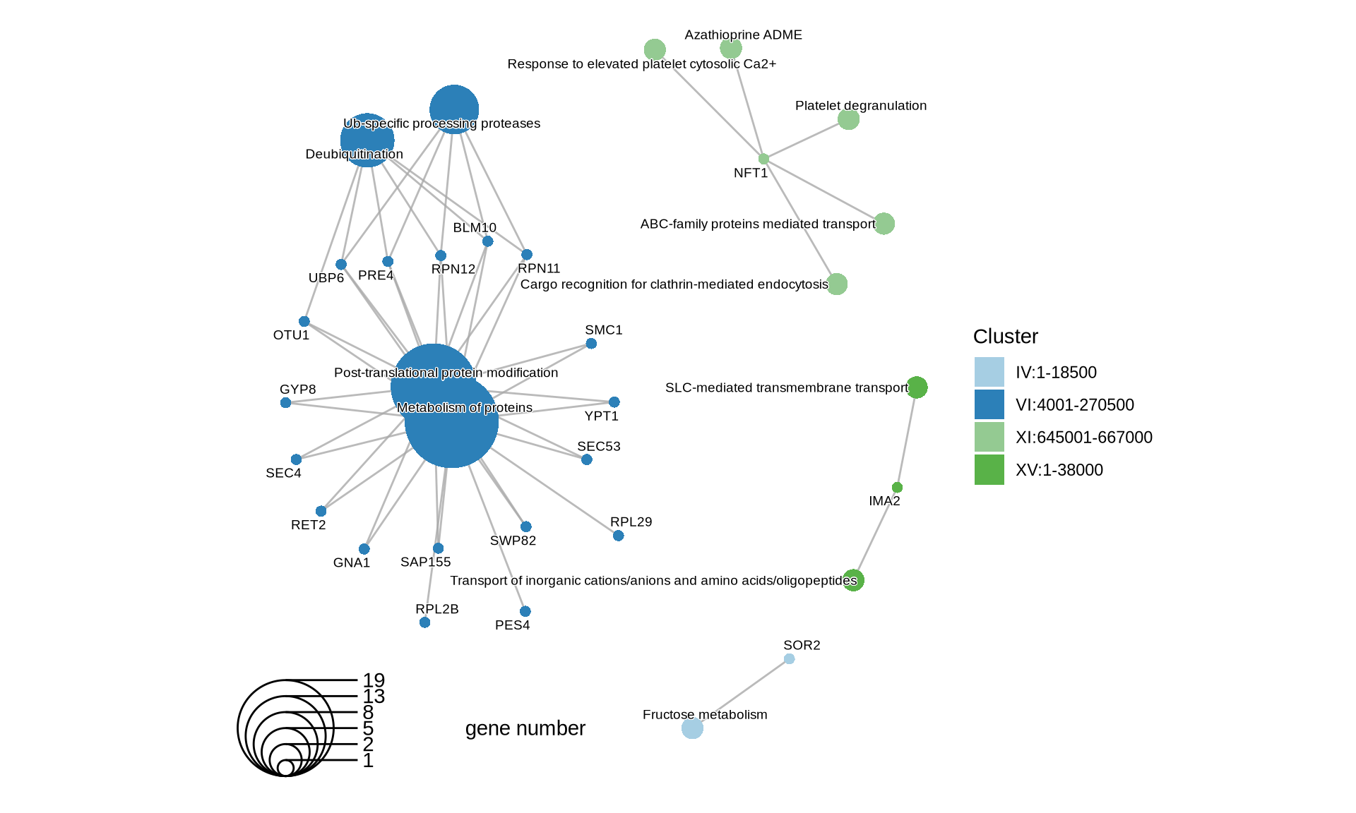
# enrich
PA = compareCluster(
  geneCluster = gene_cluster,
  fun = "enrichPathway",
  pvalueCutoff = 0.05,
  organism = ref_DB_list[[2]]
)

# map gene symbols
PA@keytype = "SYMBOL"
my_symbols = c()
for(k in 1:length(PA@geneClusters)){
  for(i in 1:length(PA@geneClusters[[k]])){
    ENTREZ = PA@geneClusters[[k]][[i]]
    SYMBOL = Scere_DB_table[which(Scere_DB_table$entrezgene_id == ENTREZ), ]$external_gene_name
    my_symbols[i] = SYMBOL
  }
  PA@geneClusters[[k]] = my_symbols
}
for(k in 1:length(PA@compareClusterResult$geneID)){
  my_vec = PA@compareClusterResult$geneID[[k]]
  my_vec = stringr::str_split(my_vec, "/")[[1]]
  for(i in 1:length(my_vec)){
    ENTREZ = my_vec[[i]]
    SYMBOL = Scere_DB_table[which(Scere_DB_table$entrezgene_id == ENTREZ), ]$external_gene_name
    my_vec[[i]] = SYMBOL[[1]]
  }
  my_vec = paste(my_vec, collapse = "/")
  PA@compareClusterResult$geneID[[k]] = my_vec
}

# plot
p1 = enrichplot::dotplot(PA, includeAll = TRUE) +
  scale_colour_gradientn(colours = rev(colorRampPalette(brewer.pal(7, "Reds"))(37))) +
  guides(colour = guide_colorbar(reverse = TRUE)) +
  theme(plot.title = element_text(size = 22, hjust = 0.5)) +
  theme(axis.text.x=element_text(angle = 45, hjust = 1))

p2 = cnetplot(PA) +
  scale_fill_manual(values = colorRampPalette(brewer.pal(10, "Paired"))(length(PA@geneClusters))) +
  theme(plot.title = element_text(size = 22, hjust = 0.5))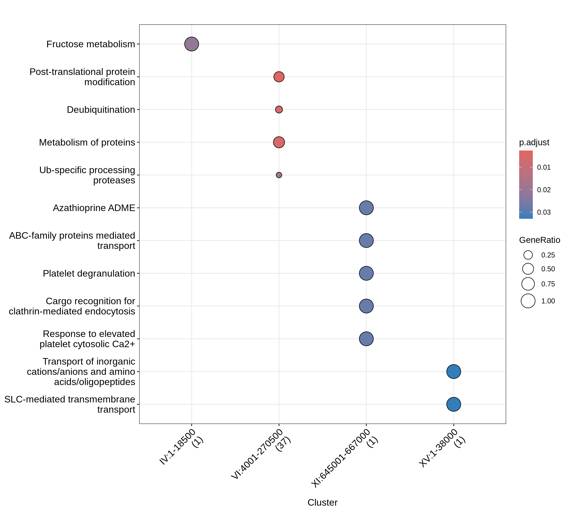
4.5 Lessons Learnt
Based on the we have learnt:
- Fr
4.6 Session Information
R version 4.3.3 (2024-02-29)
Platform: x86_64-pc-linux-gnu (64-bit)
Running under: Ubuntu 24.04.3 LTS

Matrix products: default
BLAS:   /usr/lib/x86_64-linux-gnu/blas/libblas.so.3.12.0
LAPACK: /usr/lib/x86_64-linux-gnu/lapack/liblapack.so.3.12.0

locale:
 [1] LC_CTYPE=en_US.UTF-8    LC_NUMERIC=C            LC_TIME=C
 [4] LC_COLLATE=en_US.UTF-8  LC_MONETARY=C           LC_MESSAGES=en_US.UTF-8
 [7] LC_PAPER=C              LC_NAME=C               LC_ADDRESS=C
[10] LC_TELEPHONE=C          LC_MEASUREMENT=C        LC_IDENTIFICATION=C

time zone: Europe/Brussels
tzcode source: system (glibc)

attached base packages:
[1] stats4    grid      stats     graphics  grDevices utils     datasets
[8] methods   base

other attached packages:
 [1] org.Sc.sgd.db_3.18.0   AnnotationDbi_1.64.1   IRanges_2.36.0
 [4] S4Vectors_0.40.2       Biobase_2.62.0         BiocGenerics_0.48.1
 [7] RColorBrewer_1.1-3     magrittr_2.0.3         gridExtra_2.3
[10] ggplot2_3.5.2          DT_0.33                ComplexHeatmap_2.18.0
[13] clusterProfiler_4.10.1 circlize_0.4.16

loaded via a namespace (and not attached):
  [1] jsonlite_2.0.0          shape_1.4.6.1           magick_2.8.7
  [4] farver_2.1.2            rmarkdown_2.29          GlobalOptions_0.1.2
  [7] fs_1.6.6                zlibbioc_1.48.2         vctrs_0.6.5
 [10] memoise_2.0.1           RCurl_1.98-1.17         ggtree_3.10.1
 [13] progress_1.2.3          htmltools_0.5.8.1       curl_6.4.0
 [16] gridGraphics_0.5-1      sass_0.4.10             bslib_0.9.0
 [19] htmlwidgets_1.6.4       plyr_1.8.9              cachem_1.1.0
 [22] igraph_2.1.4            lifecycle_1.0.4         iterators_1.0.14
 [25] pkgconfig_2.0.3         Matrix_1.6-5            R6_2.6.1
 [28] fastmap_1.2.0           gson_0.1.0              GenomeInfoDbData_1.2.11
 [31] clue_0.3-66             digest_0.6.37           aplot_0.2.8
 [34] enrichplot_1.22.0       colorspace_2.1-1        patchwork_1.3.1
 [37] crosstalk_1.2.1         RSQLite_2.4.2           filelock_1.0.3
 [40] labeling_0.4.3          httr_1.4.7              polyclip_1.10-7
 [43] compiler_4.3.3          bit64_4.6.0-1           withr_3.0.2
 [46] doParallel_1.0.17       graphite_1.48.0         S7_0.2.0
 [49] BiocParallel_1.36.0     viridis_0.6.5           DBI_1.2.3
 [52] ggforce_0.5.0           biomaRt_2.58.2          MASS_7.3-60.0.1
 [55] rappdirs_0.3.3          rjson_0.2.23            HDO.db_0.99.1
 [58] tools_4.3.3             ape_5.8-1               scatterpie_0.2.5
 [61] glue_1.8.0              nlme_3.1-164            GOSemSim_2.28.1
 [64] shadowtext_0.1.5        cluster_2.1.6           reshape2_1.4.4
 [67] fgsea_1.35.6            generics_0.1.4          gtable_0.3.6
 [70] tidyr_1.3.1             hms_1.1.3               data.table_1.17.8
 [73] xml2_1.3.8              tidygraph_1.3.1         XVector_0.42.0
 [76] ggrepel_0.9.6           foreach_1.5.2           pillar_1.11.0
 [79] stringr_1.5.1           yulab.utils_0.2.0       splines_4.3.3
 [82] dplyr_1.1.4             tweenr_2.0.3            BiocFileCache_2.10.2
 [85] treeio_1.26.0           lattice_0.22-5          bit_4.6.0
 [88] tidyselect_1.2.1        GO.db_3.18.0            Biostrings_2.70.3
 [91] reactome.db_1.86.2      knitr_1.50              xfun_0.52
 [94] graphlayouts_1.2.2      matrixStats_1.5.0       stringi_1.8.7
 [97] lazyeval_0.2.2          ggfun_0.2.0             yaml_2.3.10
[100] ReactomePA_1.46.0       evaluate_1.0.4          codetools_0.2-19
[103] ggraph_2.2.1            tibble_3.3.0            qvalue_2.34.0
[106] graph_1.80.0            BiocManager_1.30.26     ggplotify_0.1.2
[109] cli_3.6.5               jquerylib_0.1.4         dichromat_2.0-0.1
[112] Rcpp_1.1.0              GenomeInfoDb_1.38.8     dbplyr_2.5.0
[115] png_0.1-8               XML_3.99-0.18           parallel_4.3.3
[118] blob_1.2.4              prettyunits_1.2.0       DOSE_3.28.2
[121] bitops_1.0-9            viridisLite_0.4.2       tidytree_0.4.6
[124] scales_1.4.0            purrr_1.1.0             crayon_1.5.3
[127] GetoptLong_1.0.5        rlang_1.1.6             cowplot_1.2.0
[130] fastmatch_1.1-6         KEGGREST_1.42.0