6  High-throughput phenotyping

6.1 On this page

Biological insights and take-home messages are at the bottom of the page at section Lesson Learnt: Section 6.5.

• Here

6.2 High-throughput phenotyping of farmhouse and industrial yeasts

Let’s import the phenotypic data and reformat them.

# import and prep data
raw_data = read.delim("./data/p01-06/grouped phenotype data with annotations.csv", sep = ",", header = TRUE)

raw_data = raw_data %>%
  dplyr::filter(group != "WL004") %>%
  dplyr::filter(group != "LA001")
raw_data$Industry = ifelse(
  raw_data$region %in% c("South-West Norway", "Lithuania", "North-West Norway", "Russia",
                         "Central-Eastern Norway", "Latvia", "South-Eastern Norway"),
  "Farmhouse",
  raw_data$region
)
raw_data$Industry = ifelse(
  raw_data$Outside == "yes",
  "Allochthonous\nyeast",
  raw_data$Industry
)
raw_data$region = ifelse(
  raw_data$Industry == "Farmhouse",
  raw_data$region,
  "NA"
)

raw_data$region = ifelse(
  raw_data$culture %in% c("7", "38"),
  "South-West Norway",
  ifelse(
    raw_data$culture == "40",
    "Russia",
    ifelse(
      raw_data$culture == "45",
      "Latvia",
      ifelse(
        raw_data$culture == "57",
        "Central-Eastern Norway",
        raw_data$region
      )
    )
  )
)


raw_data = raw_data %>%
  dplyr::mutate(region = dplyr::case_when(
    region == "South-West Norway" ~ "SW Norway",
    region == "North-West Norway" ~ "NW Norway",
    region == "Central-Eastern Norway" ~ "CE Norway",
    region == "South-Eastern Norway" ~ "SE Norway",
    .default = as.character(region)
  ))

metadata = raw_data %>%
  dplyr::select(c("group", "culture", "region", "Industry", "Outside", "method"))
rownames(metadata) = metadata$group

rownames(raw_data) = raw_data$group
counts = raw_data %>%
  dplyr::select(-c("group", "culture", "region", "Industry", "Outside", "method"))

# import final clade list
final_clades = read.table(
  "./data/p01-06/final_clades_for_pub.txt",
  sep = "\t",
  header = TRUE,
  stringsAsFactors = FALSE
)
# replace
for(i in 1:nrow(final_clades)){

  strain = final_clades[i, "Strain"]
  clade = final_clades[i, "Clade"]
  metadata[which(metadata$group == strain), "Industry"] = clade

}
metadata$Industry = ifelse(metadata$Industry == "Beer", "Beer2", metadata$Industry)
metadata$Industry = ifelse(metadata$group == "BI001", "Asia", metadata$Industry)
metadata$Industry = ifelse(metadata$group == "BR003", "Mixed", metadata$Industry)
metadata$Industry = ifelse(metadata$group == "BI002", "Other", metadata$Industry)
metadata$Industry = ifelse(metadata$group == "BI004", "Asia", metadata$Industry)
metadata$Industry = ifelse(metadata$group == "BI005", "Other", metadata$Industry)


## background: no farmhouse
metadata_no_farm = metadata[which(metadata$Industry != "Farmhouse"), ]
metadata_no_farm = metadata_no_farm[which(metadata_no_farm$Industry != "Allochthonous\nyeast"), ]
counts_no_farm = counts[which(rownames(counts) %in% metadata_no_farm$group), ]

## farmhouse focus
metadata_farm_only = metadata[which(metadata$Industry %in% c("Farmhouse", "Allochthonous\nyeast")), ]
colnames(metadata_farm_only)[5] = "Allochthonous"
metadata_farm_only$Allochthonous = ifelse(metadata_farm_only$Allochthonous == "yes", "yes", "no")
counts_farm_only = counts[which(rownames(counts) %in% metadata_farm_only$group), ]

6.2.1 Principal Component Analysis

6.2.1.1 Background: no farmhouse yeasts

# create PCA object
pca_obj = PCAtools::pca(t(counts_no_farm),
                        metadata_no_farm,
                        removeVar = 0.1)


### IDENTIFY NUMBER OF SIGNIFICANT PRINCIPAL COMPONENTS
# Elbow method
elbow_method = PCAtools::findElbowPoint(pca_obj$variance)

# minimum number of components that explains 80% of variance
nPCopt = which(cumsum(pca_obj$variance) > 80)[1]

# max number of component + 1
if(elbow_method >= nPCopt){
  nPCmax = elbow_method + 1
} else{
  nPCmax= nPCopt
}

saassa

# screeplot
p1 = PCAtools::screeplot(pca_obj,
                        components = pca_obj$components[1:nPCmax],
                        vline = c(elbow_method, nPCopt),
                        colBar = rev(colorRampPalette(brewer.pal(7, "Blues"))(nPCmax)),
                        axisLabSize = 18,
                        titleLabSize = 22) +
  geom_label(aes(x = elbow_method, y = 50, label = "Elbow method", vjust = -1, size = 8)) +
  geom_label(aes(x = nPCopt, y = 50, label = "80% variance", vjust = -1, size = 8), colour = "steelblue") +
  theme(plot.title = element_blank())

p1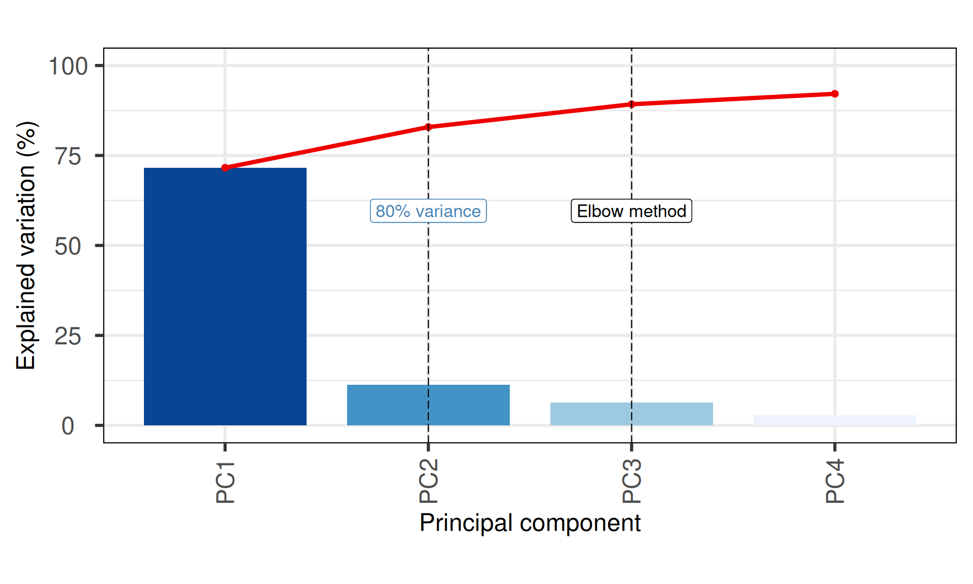

Figure 1: Screeplot of PC variants without farmhouse yeasts.

asasas

### BIPLOT
p1 = PCAtools::biplot(pca_obj,
                      labSize = 0,
                      pointSize = 5,
                      drawConnectors = FALSE,
                      max.overlaps = 700,
                      colby = "Industry",
                      colkey = c('#e6194b', '#ffe119', '#46f0f0', '#911eb4', "grey75", '#bcf60c'),
                      legendPosition = "right") +
  theme(plot.title = element_blank(),
        plot.subtitle = element_blank(),
        legend.background = element_rect(colour = "grey25", size = 0.5))
p1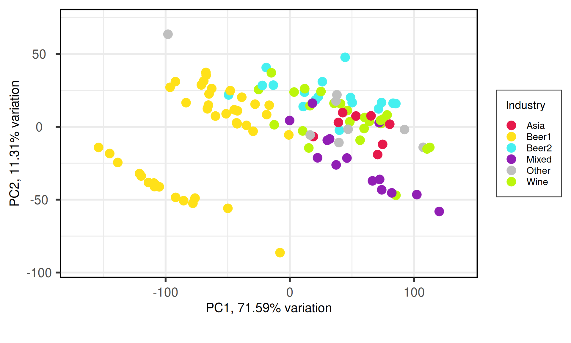

Figure 2: Biplot of industrial yests phenotypes.

saasas

## PAIRSPLOT
max_pairplot_comp = ifelse(nPCmax - 1 <= 10, nPCmax - 1, 10)
p1 = PCAtools::pairsplot(pca_obj,
                          components = pca_obj$components[1:(max_pairplot_comp)],
                          colby = "Industry",
                          colkey = c('#e6194b', '#ffe119', '#46f0f0', '#911eb4', "grey75", '#bcf60c'),
                          pointSize = 2,
                          trianglelabSize = 12,
                          plotaxes = FALSE,
                          margingaps = unit(c(0.05, 0.05, 0.05, 0.05), "cm"),
                          title = paste0("Top ", nPCmax - 1, " Principal Components")) +
  theme(plot.title = element_blank())
p1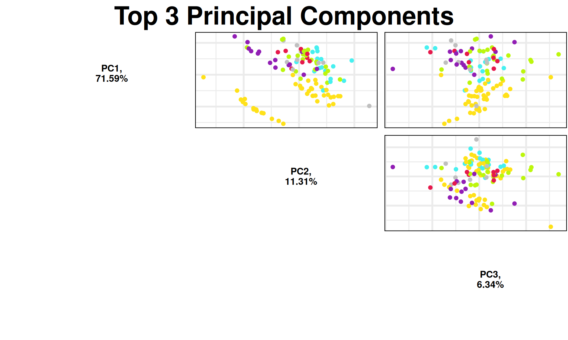

Figure 3: Biplot of industrial yests phenotypes.

### PRINCIPAL COMPONENTS LOADINGS
# plot loadings
p1 = PCAtools::plotloadings(pca_obj,
                            components = getComponents(pca_obj, seq_len(nPCmax - 1)),
                            rangeRetain = 0.01,
                            labSize = 3,
                            title = "Loadings plot: correlation between phenotypes",
                            subtitle = paste0("and the ", nPCmax - 1, " Significant Principal Components "),
                            caption = "Top 1% variables",
                            shape = 21,
                            col = c('steelblue', 'white', 'red3'),
                            drawConnectors = TRUE) +
  theme(plot.title = element_blank(),
        plot.subtitle = element_blank())
p1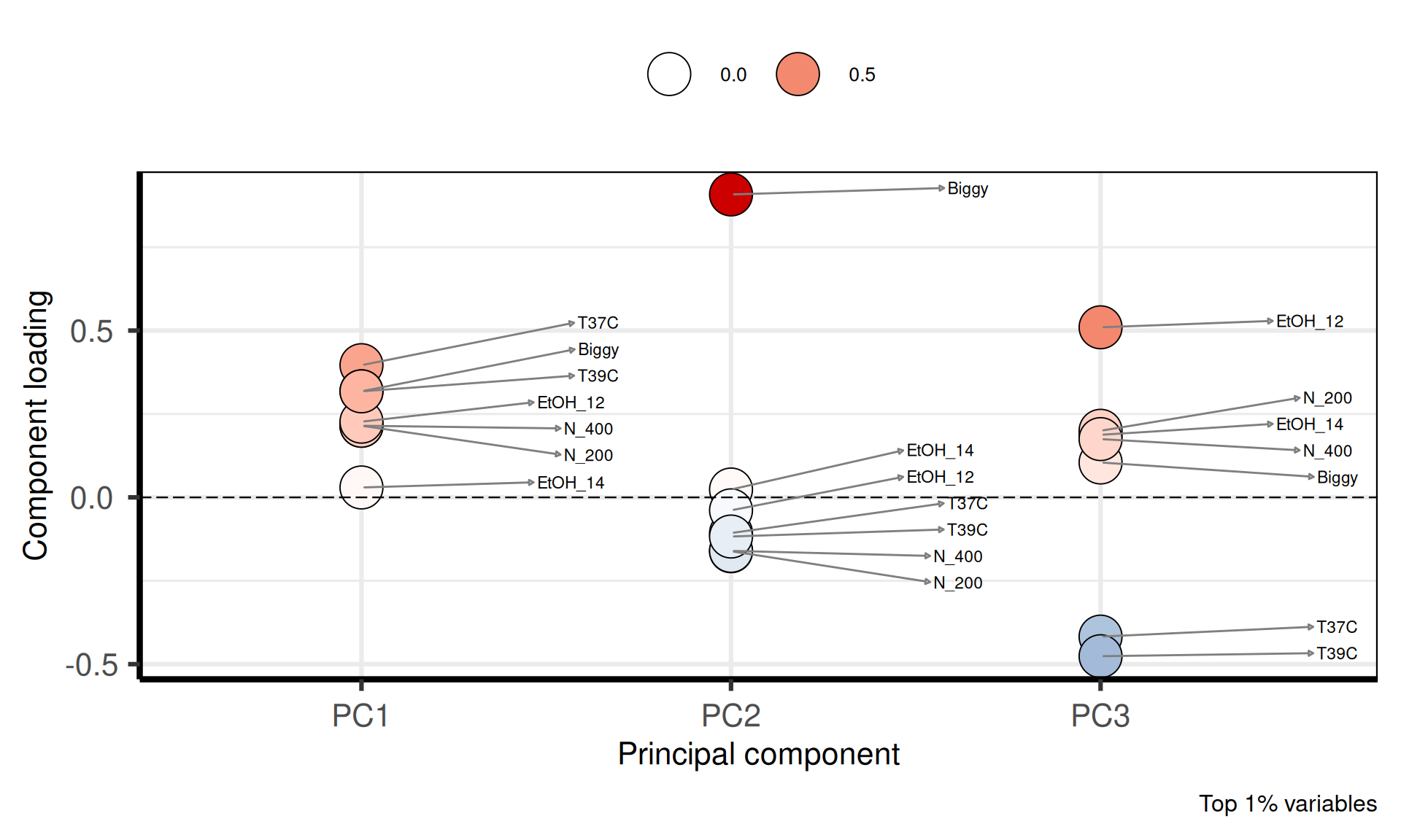

Figure 4: Industrial yests phenotypes loadings.

6.2.1.2 Farmhouse and industrial yeasts

# create PCA object
pca_obj = PCAtools::pca(t(counts),
                        metadata,
                        removeVar = 0.1)


### IDENTIFY NUMBER OF SIGNIFICANT PRINCIPAL COMPONENTS

# Elbow method
elbow_method = PCAtools::findElbowPoint(pca_obj$variance)

# minimum number of components that explains 80% of variance
nPCopt = which(cumsum(pca_obj$variance) > 80)[1]

# max number of component + 1
if(elbow_method >= nPCopt){
  nPCmax = elbow_method + 1
} else{
  nPCmax= nPCopt
}

sssss

# screeplot
p_all_scree = PCAtools::screeplot(pca_obj,
                        components = pca_obj$components[1:nPCmax],
                        vline = c(elbow_method, nPCopt),
                        title = "Screeplot - number of significant Principal Components",
                        ylab = "Explained\nVariation (%)",
                        colBar = rev(colorRampPalette(brewer.pal(7, "Blues"))(nPCmax)),
                        axisLabSize = 18,
                        titleLabSize = 22) +
  geom_label(aes(x = elbow_method, y = 50, label = "Elbow method", vjust = -1, size = 8)) +
  geom_label(aes(x = nPCopt, y = 50, label = "80% variance", vjust = -1, size = 8), colour = "steelblue") +
  theme(plot.title = element_blank(),
        axis.title.x = element_blank())
p_all_scree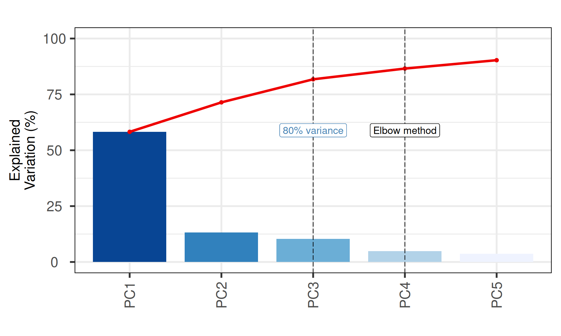

Figure 5: Screeplot of PC variants of industrial and farmhouse yeasts.

asasas

### BIPLOT
p_all_bi = PCAtools::biplot(pca_obj,
                            labSize = 0,
                            pointSize = 1.5,
                            drawConnectors = FALSE,
                            max.overlaps = 700,
                            shape ="Outside",
                            shapekey = c(20, 21),
                            colby = "Industry",
                            colkey = c("red", '#e6194b', '#ffe119', '#3cb44b', '#4363d8',  '#e6beff', '#911eb4', '#46f0f0', '#bcf60c'),
                            title = "PCA - Industry",
                            legendPosition = "right") +
  theme(plot.title = element_blank(),
        legend.background = element_rect(colour = "grey25", size = 0.5))
p_all_bi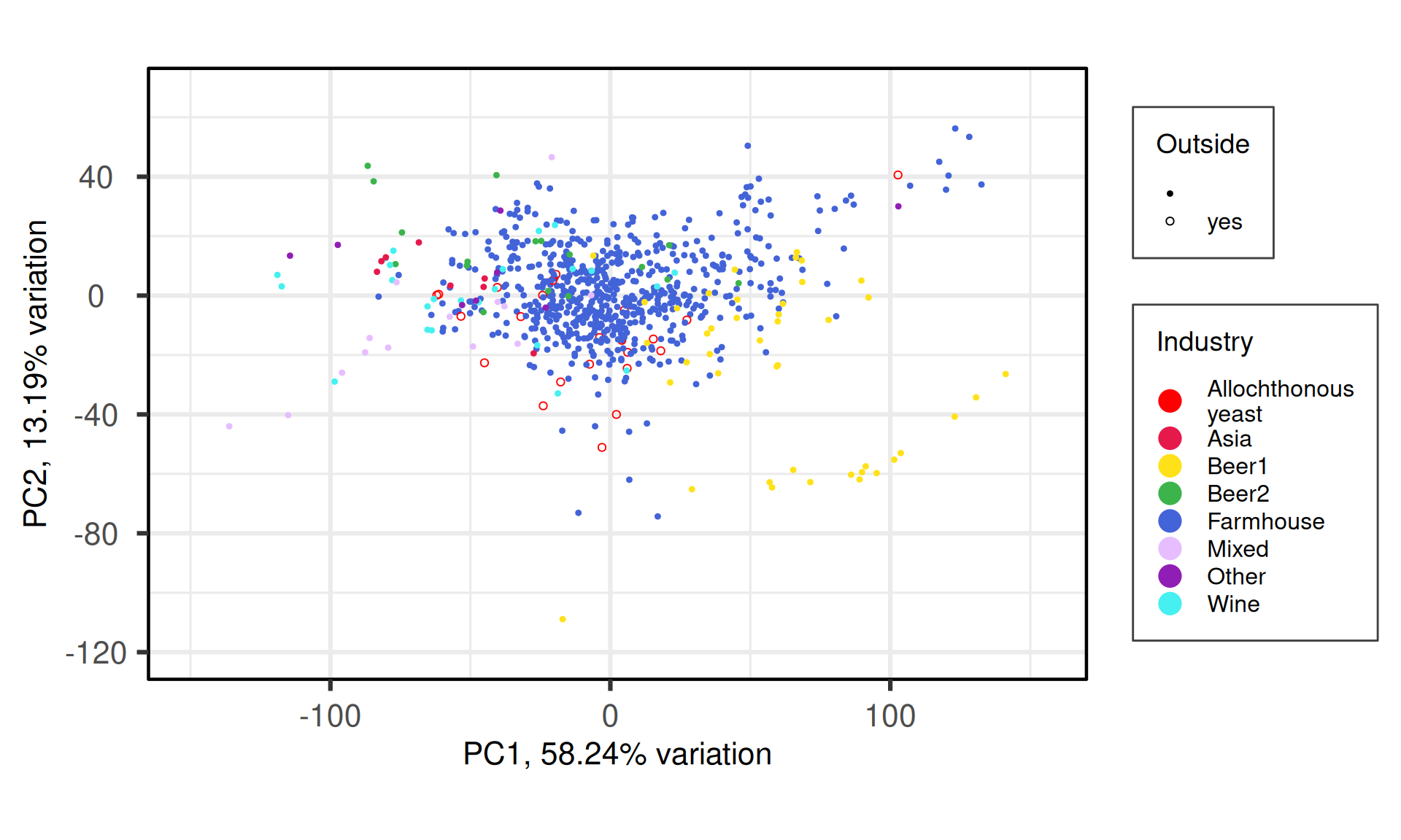

Figure 6: Biplot of framhouse and industrial yests phenotypes.

# p1 = PCAtools::biplot(pca_obj,
#                       labSize = 2,
#                       pointSize = 5,
#                       drawConnectors = TRUE,
#                       max.overlaps = 700,
#                       colby = "Industry",
#                       #colkey = c("grey75", colorRampPalette(brewer.pal(n = 4, name = "Reds"))(8)),
#                       title = "PCA - Industry",
#                       legendPosition = "bottom") +
#   theme(plot.title = element_text(size = 22, hjust = 0.5),
#         plot.subtitle = element_text(size = 18, hjust = 0.5),
#         legend.background = element_rect(colour = "grey25", size = 0.5))
# plot(p1)

## PAIRSPLOT
p_all_pair = PCAtools::pairsplot(pca_obj,
                                 components = pca_obj$components[1:4],
                                 shape ="Outside",
                                 shapekey = c(20, 21),
                                 colby = "Industry",
                                 colkey = c('#e6194b', '#ffe119', '#3cb44b', '#4363d8', "red", '#e6beff', '#911eb4', '#46f0f0', '#bcf60c'),
                                 pointSize = 1,
                                 trianglelabSize = 12,
                                 plotaxes = FALSE,
                                 margingaps = unit(c(0.05, 0.05, 0.05, 0.05), "cm")) +
  theme(plot.title = element_blank())
print(p_all_pair)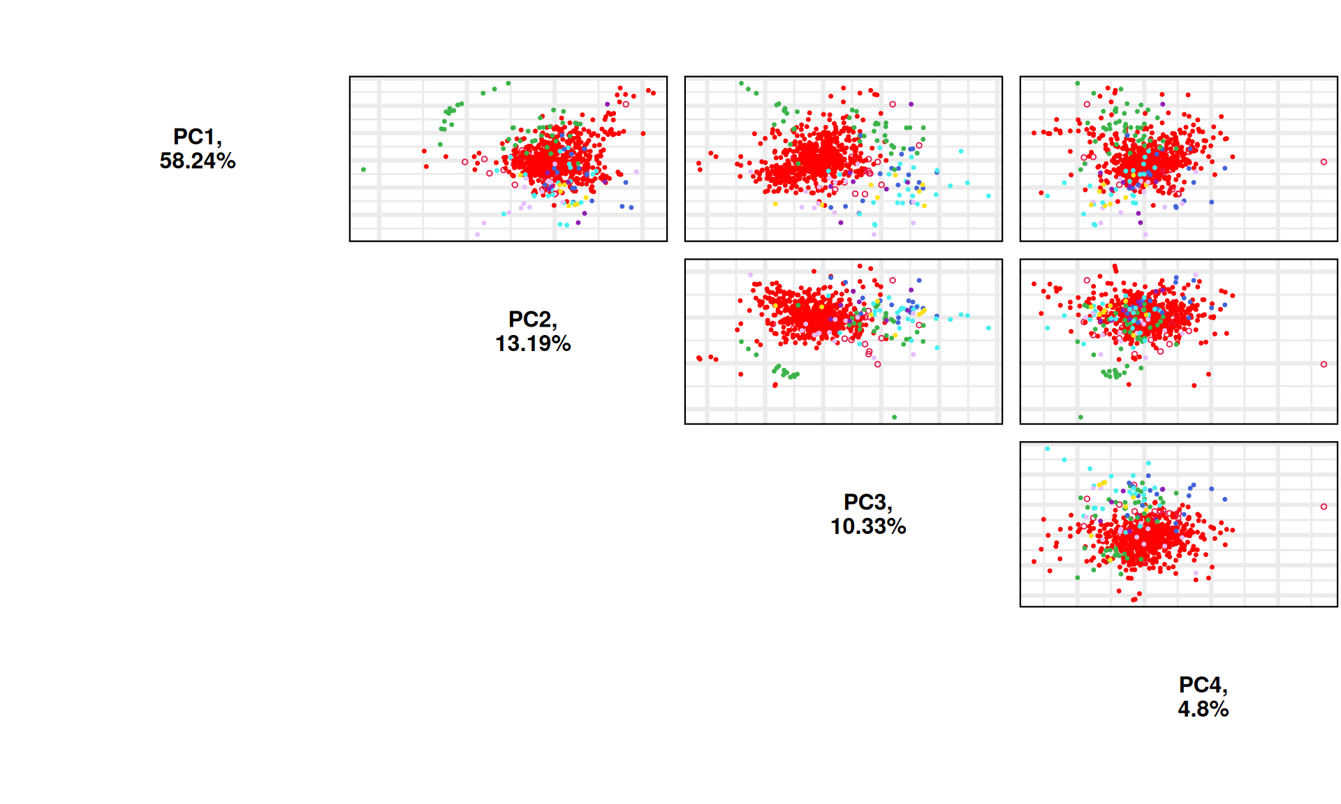

Figure 6: Biplot of framhouse and industrial yests phenotypes.

### PRINCIPAL COMPONENTS LOADINGS
# plot loadings
p_all_loads = PCAtools::plotloadings(pca_obj,
                                     components = getComponents(pca_obj, seq_len(4)),
                                     rangeRetain = 0.01,
                                     labSize = 3,
                                     caption = "Top 1% variables",
                                     shape = 21,
                                     col = c('steelblue', 'white', 'red3'),
                                     drawConnectors = TRUE) +
  theme(plot.title = element_blank(),
        plot.subtitle = element_blank(),
        legend.position = "none",
        axis.title.x = element_blank())
print(p_all_loads)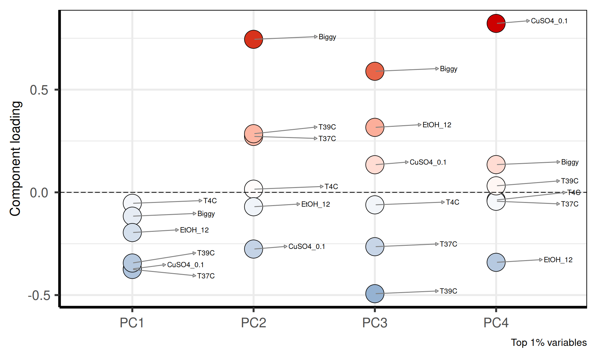

Figure 6: Biplot of framhouse and industrial yests phenotypes.

6.2.1.3 Farmhouse yeasts only

# create PCA object
pca_obj = PCAtools::pca(t(counts_farm_only),
                        metadata_farm_only,
                        removeVar = 0.1)

-- removing the lower 10% of variables based on variance

### IDENTIFY NUMBER OF SIGNIFICANT PRINCIPAL COMPONENTS
# Horn method
horn_method = tryCatch(
  PCAtools::parallelPCA(counts),
  error = function(e) { list(n = 1) }
)

Warning in check_numbers(x, k = k, nu = nu, nv = nv): more singular
values/vectors requested than available
Warning in check_numbers(x, k = k, nu = nu, nv = nv): more singular
values/vectors requested than available
Warning in check_numbers(x, k = k, nu = nu, nv = nv): more singular
values/vectors requested than available
Warning in check_numbers(x, k = k, nu = nu, nv = nv): more singular
values/vectors requested than available
Warning in check_numbers(x, k = k, nu = nu, nv = nv): more singular
values/vectors requested than available
Warning in check_numbers(x, k = k, nu = nu, nv = nv): more singular
values/vectors requested than available
Warning in check_numbers(x, k = k, nu = nu, nv = nv): more singular
values/vectors requested than available
Warning in check_numbers(x, k = k, nu = nu, nv = nv): more singular
values/vectors requested than available
Warning in check_numbers(x, k = k, nu = nu, nv = nv): more singular
values/vectors requested than available
Warning in check_numbers(x, k = k, nu = nu, nv = nv): more singular
values/vectors requested than available
Warning in check_numbers(x, k = k, nu = nu, nv = nv): more singular
values/vectors requested than available
Warning in check_numbers(x, k = k, nu = nu, nv = nv): more singular
values/vectors requested than available
Warning in check_numbers(x, k = k, nu = nu, nv = nv): more singular
values/vectors requested than available
Warning in check_numbers(x, k = k, nu = nu, nv = nv): more singular
values/vectors requested than available
Warning in check_numbers(x, k = k, nu = nu, nv = nv): more singular
values/vectors requested than available
Warning in check_numbers(x, k = k, nu = nu, nv = nv): more singular
values/vectors requested than available
Warning in check_numbers(x, k = k, nu = nu, nv = nv): more singular
values/vectors requested than available
Warning in check_numbers(x, k = k, nu = nu, nv = nv): more singular
values/vectors requested than available
Warning in check_numbers(x, k = k, nu = nu, nv = nv): more singular
values/vectors requested than available
Warning in check_numbers(x, k = k, nu = nu, nv = nv): more singular
values/vectors requested than available
Warning in check_numbers(x, k = k, nu = nu, nv = nv): more singular
values/vectors requested than available
Warning in check_numbers(x, k = k, nu = nu, nv = nv): more singular
values/vectors requested than available
Warning in check_numbers(x, k = k, nu = nu, nv = nv): more singular
values/vectors requested than available
Warning in check_numbers(x, k = k, nu = nu, nv = nv): more singular
values/vectors requested than available
Warning in check_numbers(x, k = k, nu = nu, nv = nv): more singular
values/vectors requested than available
Warning in check_numbers(x, k = k, nu = nu, nv = nv): more singular
values/vectors requested than available
Warning in check_numbers(x, k = k, nu = nu, nv = nv): more singular
values/vectors requested than available
Warning in check_numbers(x, k = k, nu = nu, nv = nv): more singular
values/vectors requested than available
Warning in check_numbers(x, k = k, nu = nu, nv = nv): more singular
values/vectors requested than available
Warning in check_numbers(x, k = k, nu = nu, nv = nv): more singular
values/vectors requested than available
Warning in check_numbers(x, k = k, nu = nu, nv = nv): more singular
values/vectors requested than available
Warning in check_numbers(x, k = k, nu = nu, nv = nv): more singular
values/vectors requested than available
Warning in check_numbers(x, k = k, nu = nu, nv = nv): more singular
values/vectors requested than available
Warning in check_numbers(x, k = k, nu = nu, nv = nv): more singular
values/vectors requested than available
Warning in check_numbers(x, k = k, nu = nu, nv = nv): more singular
values/vectors requested than available
Warning in check_numbers(x, k = k, nu = nu, nv = nv): more singular
values/vectors requested than available
Warning in check_numbers(x, k = k, nu = nu, nv = nv): more singular
values/vectors requested than available
Warning in check_numbers(x, k = k, nu = nu, nv = nv): more singular
values/vectors requested than available
Warning in check_numbers(x, k = k, nu = nu, nv = nv): more singular
values/vectors requested than available
Warning in check_numbers(x, k = k, nu = nu, nv = nv): more singular
values/vectors requested than available
Warning in check_numbers(x, k = k, nu = nu, nv = nv): more singular
values/vectors requested than available
Warning in check_numbers(x, k = k, nu = nu, nv = nv): more singular
values/vectors requested than available
Warning in check_numbers(x, k = k, nu = nu, nv = nv): more singular
values/vectors requested than available
Warning in check_numbers(x, k = k, nu = nu, nv = nv): more singular
values/vectors requested than available
Warning in check_numbers(x, k = k, nu = nu, nv = nv): more singular
values/vectors requested than available
Warning in check_numbers(x, k = k, nu = nu, nv = nv): more singular
values/vectors requested than available
Warning in check_numbers(x, k = k, nu = nu, nv = nv): more singular
values/vectors requested than available
Warning in check_numbers(x, k = k, nu = nu, nv = nv): more singular
values/vectors requested than available
Warning in check_numbers(x, k = k, nu = nu, nv = nv): more singular
values/vectors requested than available
Warning in check_numbers(x, k = k, nu = nu, nv = nv): more singular
values/vectors requested than available
Warning in check_numbers(x, k = k, nu = nu, nv = nv): more singular
values/vectors requested than available

# Elbow method
elbow_method = PCAtools::findElbowPoint(pca_obj$variance)

# minimum number of components that explains 80% of variance
nPCopt = which(cumsum(pca_obj$variance) > 80)[1]

# max number of component + 1
if(horn_method$n >= elbow_method & horn_method$n >= nPCopt){
  nPCmax = horn_method$n + 1
} else if(elbow_method >= horn_method$n & elbow_method >= nPCopt){
  nPCmax = elbow_method + 1
} else{
  nPCmax= nPCopt
}


### SCREEPLOT
# screeplot
p1 = PCAtools::screeplot(pca_obj,
                        components = pca_obj$components[1:nPCmax],
                        vline = c(horn_method$n, elbow_method, nPCopt),
                        title = "Screeplot - number of significant Principal Components",
                        colBar = rev(colorRampPalette(brewer.pal(7, "Blues"))(nPCmax)),
                        axisLabSize = 18,
                        titleLabSize = 22) +
  geom_label(aes(x = horn_method$n, y = 50, label = "Horn\'s", vjust = -1, size = 8)) +
  geom_label(aes(x = elbow_method, y = 50, label = "Elbow method", vjust = -1, size = 8)) +
  geom_label(aes(x = nPCopt, y = 50, label = "80% variance", vjust = -1, size = 8), colour = "steelblue") +
  theme(plot.title = element_text(size = 18, hjust = 0.5))
print(p1)

Warning in geom_label(aes(x = horn_method$n, y = 50, label = "Horn's", vjust = -1, : All aesthetics have length 1, but the data has 4 rows.
ℹ Please consider using `annotate()` or provide this layer with data containing
  a single row.

Warning in geom_label(aes(x = elbow_method, y = 50, label = "Elbow method", : All aesthetics have length 1, but the data has 4 rows.
ℹ Please consider using `annotate()` or provide this layer with data containing
  a single row.

Warning in geom_label(aes(x = nPCopt, y = 50, label = "80% variance", vjust = -1, : All aesthetics have length 1, but the data has 4 rows.
ℹ Please consider using `annotate()` or provide this layer with data containing
  a single row.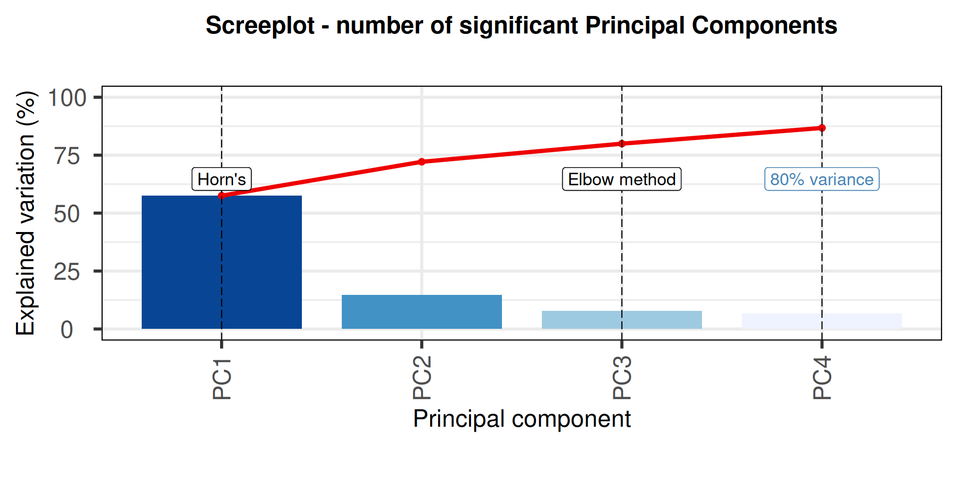

### BIPLOT
p1 = PCAtools::biplot(pca_obj,
                      labSize = 0,
                      pointSize = 2,
                      drawConnectors = FALSE,
                      max.overlaps = 700,
                      colby = "culture",
                      #colkey = c("grey75", colorRampPalette(brewer.pal(n = 4, name = "Reds"))(8)),
                      title = "PCA - culture",
                      legendPosition = "bottom") +
  theme(plot.title = element_text(size = 22, hjust = 0.5),
        plot.subtitle = element_text(size = 18, hjust = 0.5),
        legend.background = element_rect(colour = "grey25", size = 0.5))
plot(p1)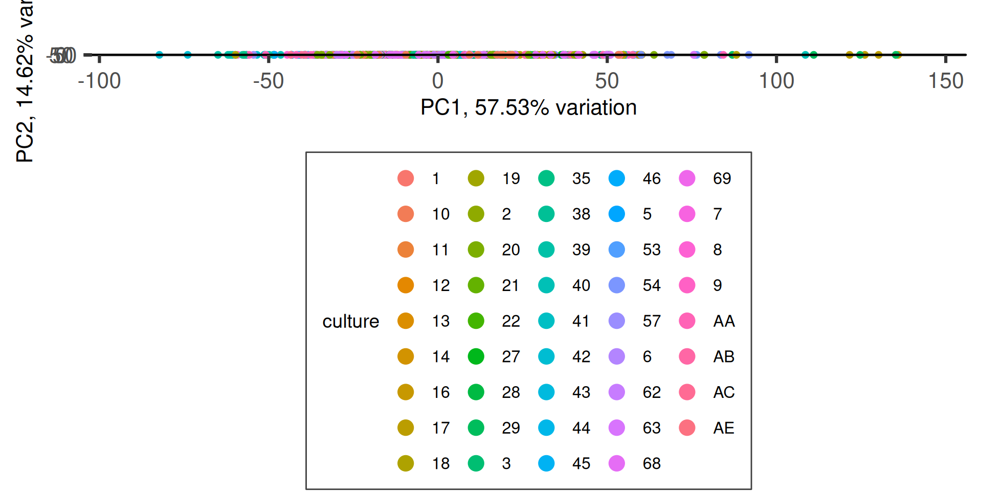

p_farm = PCAtools::biplot(pca_obj,
                          labSize = 0,
                          pointSize = 2,
                          drawConnectors = FALSE,
                          max.overlaps = 700,
                          shape ="Allochthonous",
                          shapekey = c(20, 21),
                          colby = "region",
                          colkey = c('#0571B0', '#FBA01D',"#FFDA00", "steelblue", '#A6611A',"#008470",'#92C5DE'),
                          title = "PCA - region",
                          legendPosition = "none") +
  theme(plot.title = element_blank(),
        plot.subtitle = element_blank(),
        legend.background = element_rect(colour = "grey25", size = 0.5))

Scale for colour is already present.
Adding another scale for colour, which will replace the existing scale.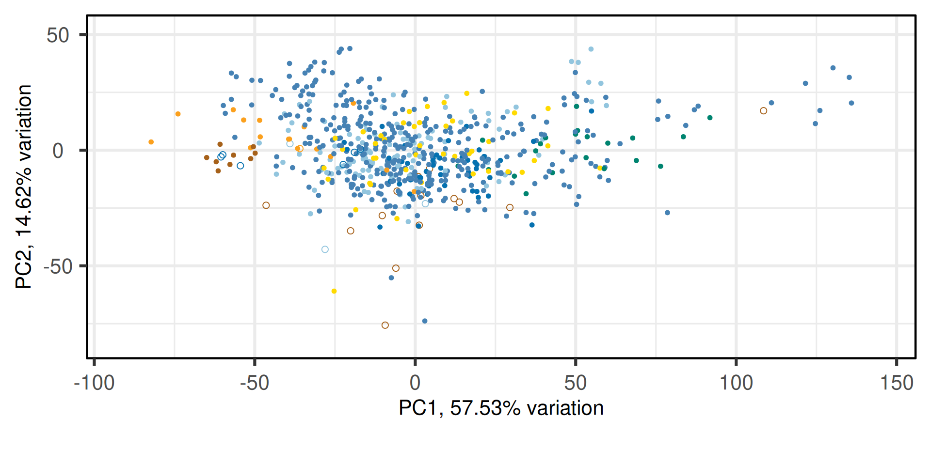

plot(p_farm)

p_farm_pair = PCAtools::pairsplot(pca_obj,
                                  components = pca_obj$components[1:4],
                                  colby = "region",
                                  shape ="Allochthonous",
                                  shapekey = c(20, 21),
                                  colkey = c('#0571B0', '#FBA01D',"#FFDA00", "steelblue", '#A6611A',"#008470",'#92C5DE'),
                                  pointSize = 1,
                                  trianglelabSize = 12,
                                  plotaxes = FALSE,
                                  margingaps = unit(c(0.05, 0.05, 0.05, 0.05), "cm")) +
  theme(plot.title = element_blank())

Scale for colour is already present.
Adding another scale for colour, which will replace the existing scale.

Scale for colour is already present.
Adding another scale for colour, which will replace the existing scale.
Scale for colour is already present.
Adding another scale for colour, which will replace the existing scale.
Scale for colour is already present.
Adding another scale for colour, which will replace the existing scale.
Scale for colour is already present.
Adding another scale for colour, which will replace the existing scale.
Scale for colour is already present.
Adding another scale for colour, which will replace the existing scale.
Coordinate system already present. Adding new coordinate system, which will
replace the existing one.
Coordinate system already present. Adding new coordinate system, which will
replace the existing one.
Coordinate system already present. Adding new coordinate system, which will
replace the existing one.
Coordinate system already present. Adding new coordinate system, which will
replace the existing one.
Coordinate system already present. Adding new coordinate system, which will
replace the existing one.
Coordinate system already present. Adding new coordinate system, which will
replace the existing one.
Coordinate system already present. Adding new coordinate system, which will
replace the existing one.
Coordinate system already present. Adding new coordinate system, which will
replace the existing one.
Coordinate system already present. Adding new coordinate system, which will
replace the existing one.
Coordinate system already present. Adding new coordinate system, which will
replace the existing one.
Coordinate system already present. Adding new coordinate system, which will
replace the existing one.
Coordinate system already present. Adding new coordinate system, which will
replace the existing one.
Coordinate system already present. Adding new coordinate system, which will
replace the existing one.
Coordinate system already present. Adding new coordinate system, which will
replace the existing one.
Coordinate system already present. Adding new coordinate system, which will
replace the existing one.
Coordinate system already present. Adding new coordinate system, which will
replace the existing one.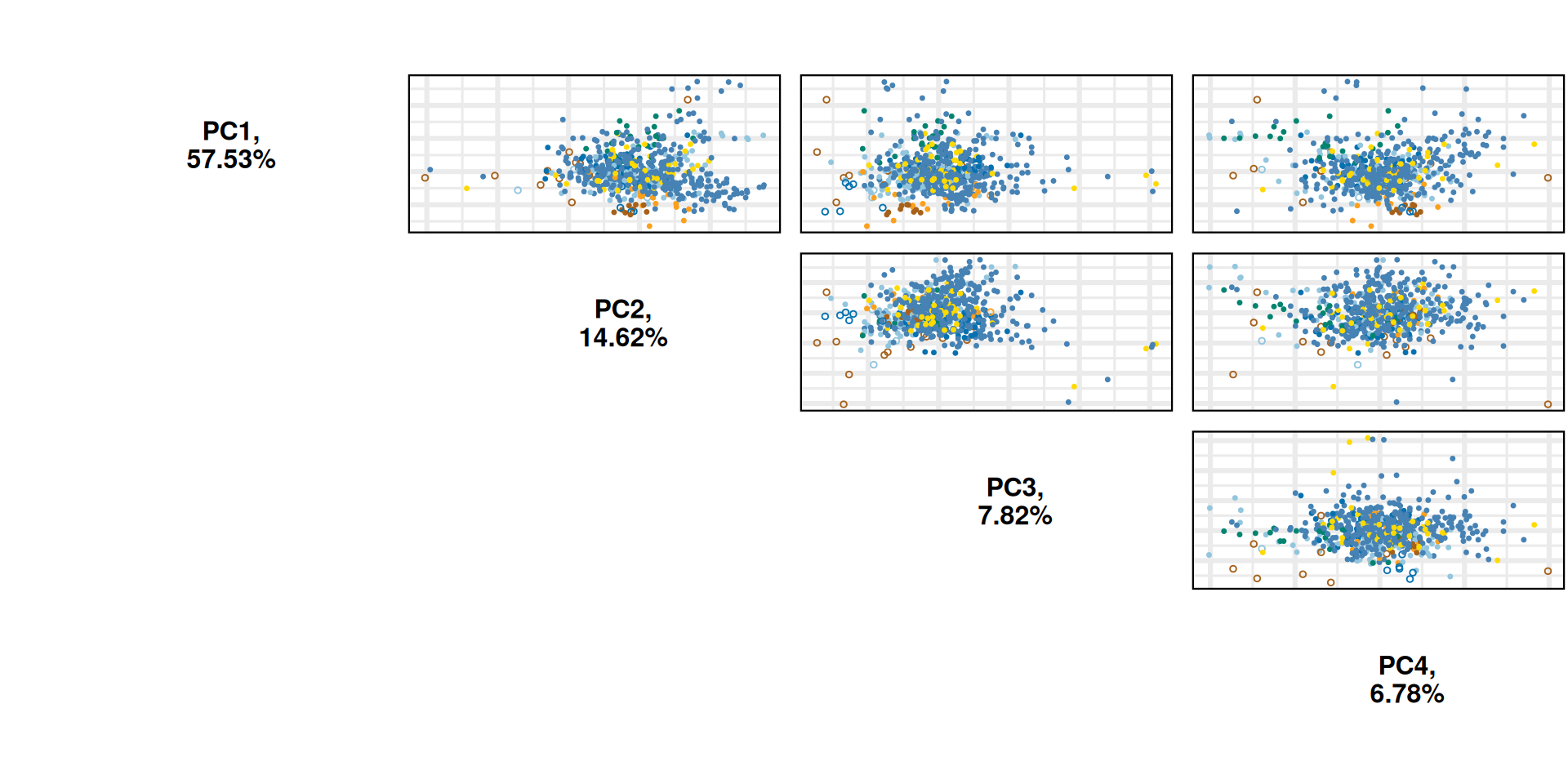

print(p_farm_pair)

p1 = PCAtools::biplot(pca_obj,
                      labSize = 0,
                      pointSize = 2,
                      drawConnectors = FALSE,
                      max.overlaps = 700,
                      colby = "method",
                      colkey = c("grey75", "firebrick", "steelblue"),
                      title = "PCA - preservation",
                      legendPosition = "bottom") +
  theme(plot.title = element_text(size = 22, hjust = 0.5),
        plot.subtitle = element_text(size = 18, hjust = 0.5),
        legend.background = element_rect(colour = "grey25", size = 0.5))

Scale for colour is already present.
Adding another scale for colour, which will replace the existing scale.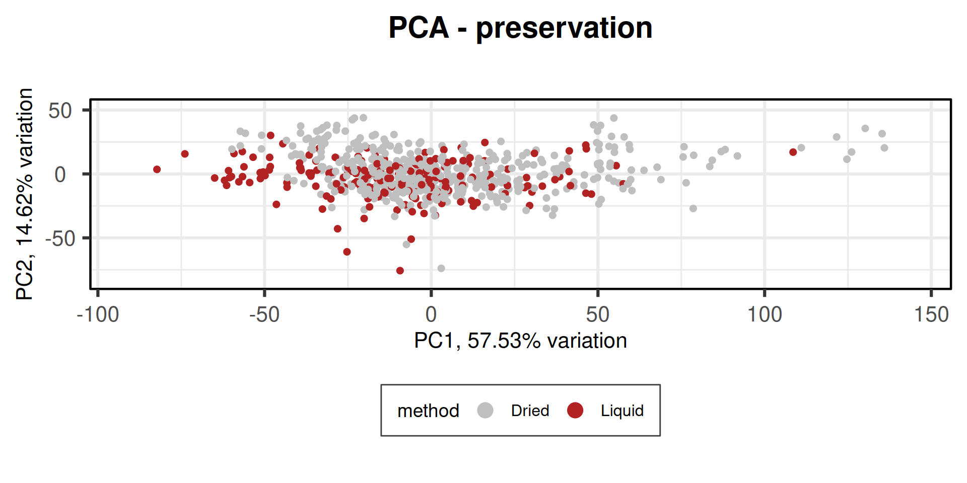

plot(p1)

p1 = PCAtools::pairsplot(pca_obj,
                          components = pca_obj$components[1:10],
                          colby = "method",
                          colkey = c("grey75", "firebrick", "steelblue"),
                          pointSize = 1,
                          trianglelabSize = 12,
                          plotaxes = FALSE,
                          margingaps = unit(c(0.05, 0.05, 0.05, 0.05), "cm")) +
  theme(plot.title = element_blank())

Scale for colour is already present.
Adding another scale for colour, which will replace the existing scale.
Scale for colour is already present.
Adding another scale for colour, which will replace the existing scale.
Scale for colour is already present.
Adding another scale for colour, which will replace the existing scale.
Scale for colour is already present.
Adding another scale for colour, which will replace the existing scale.
Scale for colour is already present.
Adding another scale for colour, which will replace the existing scale.
Scale for colour is already present.
Adding another scale for colour, which will replace the existing scale.
Scale for colour is already present.
Adding another scale for colour, which will replace the existing scale.
Scale for colour is already present.
Adding another scale for colour, which will replace the existing scale.
Scale for colour is already present.
Adding another scale for colour, which will replace the existing scale.
Scale for colour is already present.
Adding another scale for colour, which will replace the existing scale.
Scale for colour is already present.
Adding another scale for colour, which will replace the existing scale.
Scale for colour is already present.
Adding another scale for colour, which will replace the existing scale.
Scale for colour is already present.
Adding another scale for colour, which will replace the existing scale.
Scale for colour is already present.
Adding another scale for colour, which will replace the existing scale.
Scale for colour is already present.
Adding another scale for colour, which will replace the existing scale.
Scale for colour is already present.
Adding another scale for colour, which will replace the existing scale.
Scale for colour is already present.
Adding another scale for colour, which will replace the existing scale.
Scale for colour is already present.
Adding another scale for colour, which will replace the existing scale.
Scale for colour is already present.
Adding another scale for colour, which will replace the existing scale.
Scale for colour is already present.
Adding another scale for colour, which will replace the existing scale.
Scale for colour is already present.
Adding another scale for colour, which will replace the existing scale.
Scale for colour is already present.
Adding another scale for colour, which will replace the existing scale.
Scale for colour is already present.
Adding another scale for colour, which will replace the existing scale.
Scale for colour is already present.
Adding another scale for colour, which will replace the existing scale.
Scale for colour is already present.
Adding another scale for colour, which will replace the existing scale.
Scale for colour is already present.
Adding another scale for colour, which will replace the existing scale.
Scale for colour is already present.
Adding another scale for colour, which will replace the existing scale.
Scale for colour is already present.
Adding another scale for colour, which will replace the existing scale.
Scale for colour is already present.
Adding another scale for colour, which will replace the existing scale.
Scale for colour is already present.
Adding another scale for colour, which will replace the existing scale.
Scale for colour is already present.
Adding another scale for colour, which will replace the existing scale.
Scale for colour is already present.
Adding another scale for colour, which will replace the existing scale.
Scale for colour is already present.
Adding another scale for colour, which will replace the existing scale.
Scale for colour is already present.
Adding another scale for colour, which will replace the existing scale.
Scale for colour is already present.
Adding another scale for colour, which will replace the existing scale.
Scale for colour is already present.
Adding another scale for colour, which will replace the existing scale.
Scale for colour is already present.
Adding another scale for colour, which will replace the existing scale.
Scale for colour is already present.
Adding another scale for colour, which will replace the existing scale.
Scale for colour is already present.
Adding another scale for colour, which will replace the existing scale.
Scale for colour is already present.
Adding another scale for colour, which will replace the existing scale.
Scale for colour is already present.
Adding another scale for colour, which will replace the existing scale.
Scale for colour is already present.
Adding another scale for colour, which will replace the existing scale.
Scale for colour is already present.
Adding another scale for colour, which will replace the existing scale.
Scale for colour is already present.
Adding another scale for colour, which will replace the existing scale.
Scale for colour is already present.
Adding another scale for colour, which will replace the existing scale.
Coordinate system already present. Adding new coordinate system, which will
replace the existing one.
Coordinate system already present. Adding new coordinate system, which will
replace the existing one.
Coordinate system already present. Adding new coordinate system, which will
replace the existing one.
Coordinate system already present. Adding new coordinate system, which will
replace the existing one.
Coordinate system already present. Adding new coordinate system, which will
replace the existing one.
Coordinate system already present. Adding new coordinate system, which will
replace the existing one.
Coordinate system already present. Adding new coordinate system, which will
replace the existing one.
Coordinate system already present. Adding new coordinate system, which will
replace the existing one.
Coordinate system already present. Adding new coordinate system, which will
replace the existing one.
Coordinate system already present. Adding new coordinate system, which will
replace the existing one.
Coordinate system already present. Adding new coordinate system, which will
replace the existing one.
Coordinate system already present. Adding new coordinate system, which will
replace the existing one.
Coordinate system already present. Adding new coordinate system, which will
replace the existing one.
Coordinate system already present. Adding new coordinate system, which will
replace the existing one.
Coordinate system already present. Adding new coordinate system, which will
replace the existing one.
Coordinate system already present. Adding new coordinate system, which will
replace the existing one.
Coordinate system already present. Adding new coordinate system, which will
replace the existing one.
Coordinate system already present. Adding new coordinate system, which will
replace the existing one.
Coordinate system already present. Adding new coordinate system, which will
replace the existing one.
Coordinate system already present. Adding new coordinate system, which will
replace the existing one.
Coordinate system already present. Adding new coordinate system, which will
replace the existing one.
Coordinate system already present. Adding new coordinate system, which will
replace the existing one.
Coordinate system already present. Adding new coordinate system, which will
replace the existing one.
Coordinate system already present. Adding new coordinate system, which will
replace the existing one.
Coordinate system already present. Adding new coordinate system, which will
replace the existing one.
Coordinate system already present. Adding new coordinate system, which will
replace the existing one.
Coordinate system already present. Adding new coordinate system, which will
replace the existing one.
Coordinate system already present. Adding new coordinate system, which will
replace the existing one.
Coordinate system already present. Adding new coordinate system, which will
replace the existing one.
Coordinate system already present. Adding new coordinate system, which will
replace the existing one.
Coordinate system already present. Adding new coordinate system, which will
replace the existing one.
Coordinate system already present. Adding new coordinate system, which will
replace the existing one.
Coordinate system already present. Adding new coordinate system, which will
replace the existing one.
Coordinate system already present. Adding new coordinate system, which will
replace the existing one.
Coordinate system already present. Adding new coordinate system, which will
replace the existing one.
Coordinate system already present. Adding new coordinate system, which will
replace the existing one.
Coordinate system already present. Adding new coordinate system, which will
replace the existing one.
Coordinate system already present. Adding new coordinate system, which will
replace the existing one.
Coordinate system already present. Adding new coordinate system, which will
replace the existing one.
Coordinate system already present. Adding new coordinate system, which will
replace the existing one.
Coordinate system already present. Adding new coordinate system, which will
replace the existing one.
Coordinate system already present. Adding new coordinate system, which will
replace the existing one.
Coordinate system already present. Adding new coordinate system, which will
replace the existing one.
Coordinate system already present. Adding new coordinate system, which will
replace the existing one.
Coordinate system already present. Adding new coordinate system, which will
replace the existing one.
Coordinate system already present. Adding new coordinate system, which will
replace the existing one.
Coordinate system already present. Adding new coordinate system, which will
replace the existing one.
Coordinate system already present. Adding new coordinate system, which will
replace the existing one.
Coordinate system already present. Adding new coordinate system, which will
replace the existing one.
Coordinate system already present. Adding new coordinate system, which will
replace the existing one.
Coordinate system already present. Adding new coordinate system, which will
replace the existing one.
Coordinate system already present. Adding new coordinate system, which will
replace the existing one.
Coordinate system already present. Adding new coordinate system, which will
replace the existing one.
Coordinate system already present. Adding new coordinate system, which will
replace the existing one.
Coordinate system already present. Adding new coordinate system, which will
replace the existing one.
Coordinate system already present. Adding new coordinate system, which will
replace the existing one.
Coordinate system already present. Adding new coordinate system, which will
replace the existing one.
Coordinate system already present. Adding new coordinate system, which will
replace the existing one.
Coordinate system already present. Adding new coordinate system, which will
replace the existing one.
Coordinate system already present. Adding new coordinate system, which will
replace the existing one.
Coordinate system already present. Adding new coordinate system, which will
replace the existing one.
Coordinate system already present. Adding new coordinate system, which will
replace the existing one.
Coordinate system already present. Adding new coordinate system, which will
replace the existing one.
Coordinate system already present. Adding new coordinate system, which will
replace the existing one.
Coordinate system already present. Adding new coordinate system, which will
replace the existing one.
Coordinate system already present. Adding new coordinate system, which will
replace the existing one.
Coordinate system already present. Adding new coordinate system, which will
replace the existing one.
Coordinate system already present. Adding new coordinate system, which will
replace the existing one.
Coordinate system already present. Adding new coordinate system, which will
replace the existing one.
Coordinate system already present. Adding new coordinate system, which will
replace the existing one.
Coordinate system already present. Adding new coordinate system, which will
replace the existing one.
Coordinate system already present. Adding new coordinate system, which will
replace the existing one.
Coordinate system already present. Adding new coordinate system, which will
replace the existing one.
Coordinate system already present. Adding new coordinate system, which will
replace the existing one.
Coordinate system already present. Adding new coordinate system, which will
replace the existing one.
Coordinate system already present. Adding new coordinate system, which will
replace the existing one.
Coordinate system already present. Adding new coordinate system, which will
replace the existing one.
Coordinate system already present. Adding new coordinate system, which will
replace the existing one.
Coordinate system already present. Adding new coordinate system, which will
replace the existing one.
Coordinate system already present. Adding new coordinate system, which will
replace the existing one.
Coordinate system already present. Adding new coordinate system, which will
replace the existing one.
Coordinate system already present. Adding new coordinate system, which will
replace the existing one.
Coordinate system already present. Adding new coordinate system, which will
replace the existing one.
Coordinate system already present. Adding new coordinate system, which will
replace the existing one.
Coordinate system already present. Adding new coordinate system, which will
replace the existing one.
Coordinate system already present. Adding new coordinate system, which will
replace the existing one.
Coordinate system already present. Adding new coordinate system, which will
replace the existing one.
Coordinate system already present. Adding new coordinate system, which will
replace the existing one.
Coordinate system already present. Adding new coordinate system, which will
replace the existing one.
Coordinate system already present. Adding new coordinate system, which will
replace the existing one.
Coordinate system already present. Adding new coordinate system, which will
replace the existing one.
Coordinate system already present. Adding new coordinate system, which will
replace the existing one.
Coordinate system already present. Adding new coordinate system, which will
replace the existing one.
Coordinate system already present. Adding new coordinate system, which will
replace the existing one.
Coordinate system already present. Adding new coordinate system, which will
replace the existing one.
Coordinate system already present. Adding new coordinate system, which will
replace the existing one.
Coordinate system already present. Adding new coordinate system, which will
replace the existing one.
Coordinate system already present. Adding new coordinate system, which will
replace the existing one.
Coordinate system already present. Adding new coordinate system, which will
replace the existing one.
Coordinate system already present. Adding new coordinate system, which will
replace the existing one.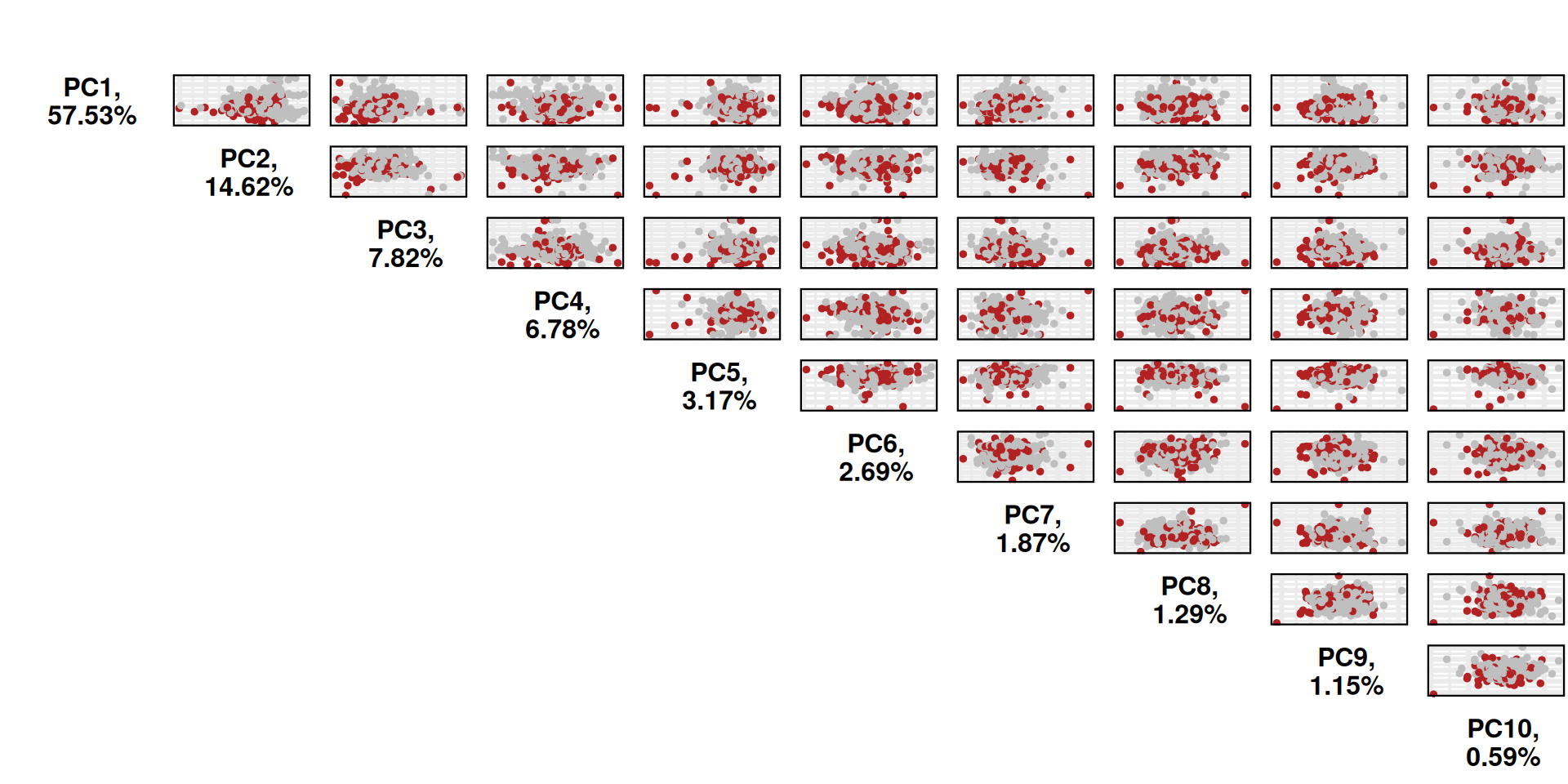

print(p1)

### PRINCIPAL COMPONENTS LOADINGS
# plot loadings
p1 = PCAtools::plotloadings(pca_obj,
                            components = getComponents(pca_obj, seq_len(nPCmax - 1)),
                            rangeRetain = 0.01,
                            labSize = 3,
                            title = "Loadings plot: correlation between phenotypes",
                            subtitle = paste0("and the ", nPCmax - 1, " Significant Principal Components "),
                            caption = "Top 1% variables",
                            shape = 21,
                            col = c('steelblue', 'white', 'red3'),
                            drawConnectors = TRUE) +
  theme(plot.title = element_text(size = 22, hjust = 0.5),
        plot.subtitle = element_text(size = 18, hjust = 0.5))

-- variables retained:
Biggy, CuSO4_0.1, T39C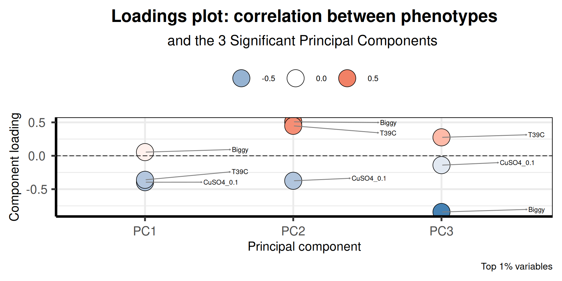

print(p1)

6.2.2 Discriminant analysis

sPLS-DA

6.3 FArmhouse

6.3.1 PCA

6.3.2 Distributions

6.4 Fermentations

6.5 Lessons Learnt

Based on the we have learnt:

• Fr

6.6 Session Information

Note

R version 4.3.3 (2024-02-29)
Platform: x86_64-pc-linux-gnu (64-bit)
Running under: Ubuntu 24.04.3 LTS

Matrix products: default
BLAS:   /usr/lib/x86_64-linux-gnu/blas/libblas.so.3.12.0 
LAPACK: /usr/lib/x86_64-linux-gnu/lapack/liblapack.so.3.12.0

locale:
 [1] LC_CTYPE=en_US.UTF-8    LC_NUMERIC=C            LC_TIME=C              
 [4] LC_COLLATE=en_US.UTF-8  LC_MONETARY=C           LC_MESSAGES=en_US.UTF-8
 [7] LC_PAPER=C              LC_NAME=C               LC_ADDRESS=C           
[10] LC_TELEPHONE=C          LC_MEASUREMENT=C        LC_IDENTIFICATION=C    

time zone: Europe/Brussels
tzcode source: system (glibc)

attached base packages:
[1] grid      stats     graphics  grDevices utils     datasets  methods  
[8] base     

other attached packages:
 [1] treeio_1.26.0      stringr_1.5.1      reshape2_1.4.4     reshape_0.8.10    
 [5] RColorBrewer_1.1-3 plyr_1.8.9         phytools_2.4-4     maps_3.4.3        
 [9] PCAtools_2.14.0    ggrepel_0.9.6      naturalsort_0.1.3  mixOmics_6.26.0   
[13] lattice_0.22-5     MASS_7.3-60.0.1    gtable_0.3.6       gridExtra_2.3     
[17] ggtreeExtra_1.12.0 ggtree_3.10.1      ggpubr_0.6.1       ggplot2_3.5.2     
[21] ggnewscale_0.5.2   dplyr_1.1.4        aplot_0.2.8        ape_5.8-1         

loaded via a namespace (and not attached):
 [1] mnormt_2.1.1              phangorn_2.12.1          
 [3] rlang_1.1.6               magrittr_2.0.3           
 [5] matrixStats_1.5.0         compiler_4.3.3           
 [7] DelayedMatrixStats_1.24.0 vctrs_0.6.5              
 [9] combinat_0.0-8            quadprog_1.5-8           
[11] pkgconfig_2.0.3           crayon_1.5.3             
[13] fastmap_1.2.0             backports_1.5.0          
[15] XVector_0.42.0            labeling_0.4.3           
[17] rmarkdown_2.29            purrr_1.1.0              
[19] xfun_0.52                 zlibbioc_1.48.2          
[21] beachmat_2.18.1           clusterGeneration_1.3.8  
[23] jsonlite_2.0.0            DelayedArray_0.28.0      
[25] BiocParallel_1.36.0       broom_1.0.9              
[27] irlba_2.3.5.1             parallel_4.3.3           
[29] R6_2.6.1                  stringi_1.8.7            
[31] car_3.1-3                 numDeriv_2016.8-1.1      
[33] iterators_1.0.14          Rcpp_1.1.0               
[35] knitr_1.50                optimParallel_1.0-2      
[37] IRanges_2.36.0            Matrix_1.6-5             
[39] igraph_2.1.4              tidyselect_1.2.1         
[41] dichromat_2.0-0.1         abind_1.4-8              
[43] yaml_2.3.10               doParallel_1.0.17        
[45] codetools_0.2-19          tibble_3.3.0             
[47] withr_3.0.2               rARPACK_0.11-0           
[49] coda_0.19-4.1             evaluate_1.0.4           
[51] gridGraphics_0.5-1        pillar_1.11.0            
[53] MatrixGenerics_1.14.0     carData_3.0-5            
[55] foreach_1.5.2             stats4_4.3.3             
[57] ellipse_0.5.0             ggfun_0.2.0              
[59] generics_0.1.4            S4Vectors_0.40.2         
[61] sparseMatrixStats_1.14.0  scales_1.4.0             
[63] tidytree_0.4.6            glue_1.8.0               
[65] scatterplot3d_0.3-44      lazyeval_0.2.2           
[67] tools_4.3.3               ScaledMatrix_1.10.0      
[69] RSpectra_0.16-2           ggsignif_0.6.4           
[71] fs_1.6.6                  fastmatch_1.1-6          
[73] cowplot_1.2.0             tidyr_1.3.1              
[75] nlme_3.1-164              patchwork_1.3.1          
[77] BiocSingular_1.18.0       Formula_1.2-5            
[79] cli_3.6.5                 rsvd_1.0.5               
[81] DEoptim_2.2-8             expm_1.0-0               
[83] S4Arrays_1.2.1            corpcor_1.6.10           
[85] rstatix_0.7.2             yulab.utils_0.2.0        
[87] digest_0.6.37             BiocGenerics_0.48.1      
[89] SparseArray_1.2.4         ggplotify_0.1.2          
[91] dqrng_0.4.1               htmlwidgets_1.6.4        
[93] farver_2.1.2              htmltools_0.5.8.1        
[95] lifecycle_1.0.4