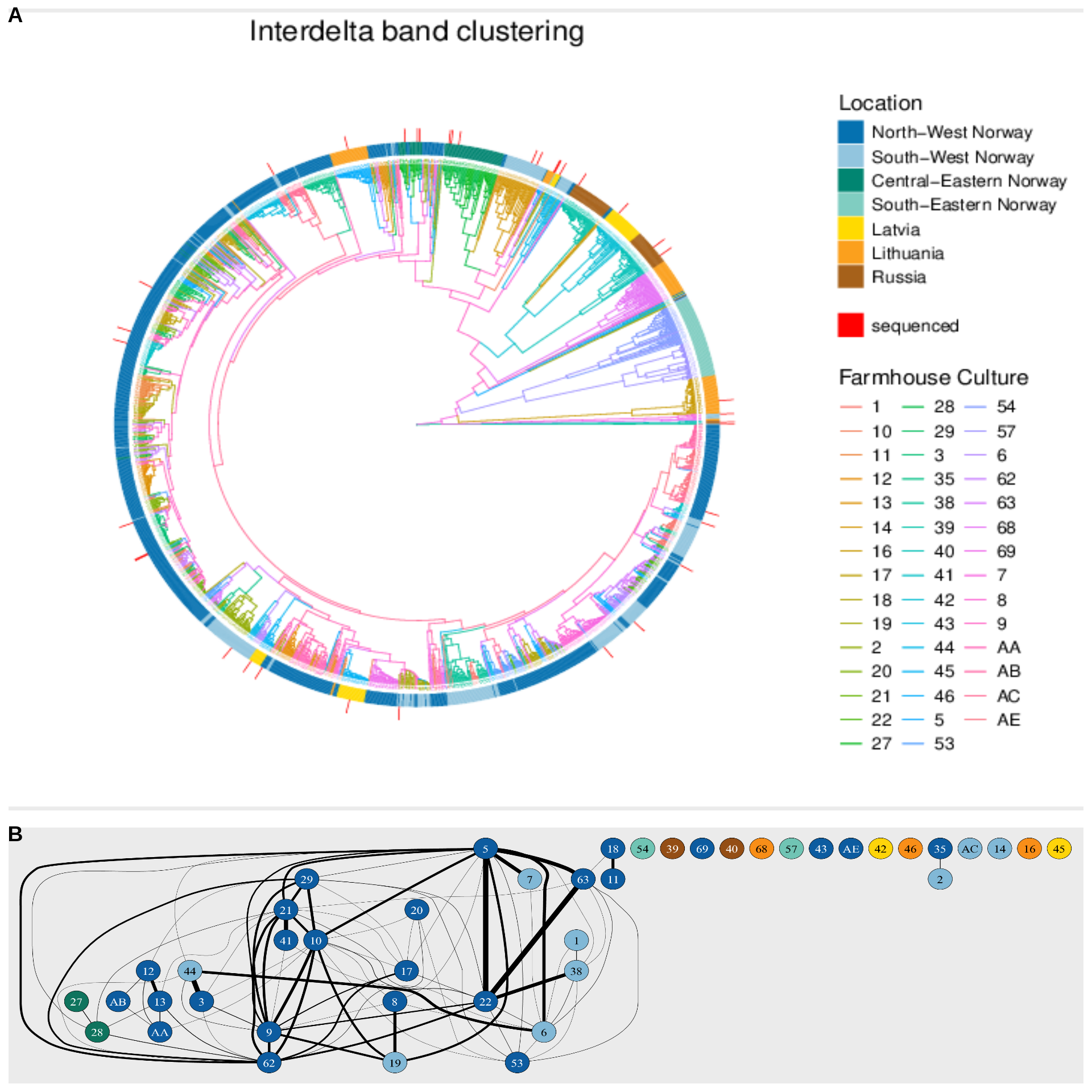
8 Figure 2
8.1 Figure 2 code
8.1.1 Panel A code
library(ape)
library(ggtree)
library(ggplot2)
library(RColorBrewer)

# Read tree in newick format using ape
kveik_tree <- read.tree('DendroExport_densitybased.txt')
# Identify tip labels that start with "AR" or "AP" as we dont have phenotype data for culture A
#tips_to_drop <- kveik_tree$tip.label[grep("^(AR|AP)", kveik_tree$tip.label)]

# rename A to AB
kveik_tree$tip.label <- sub("^AR([0-9]+)$", "ABR\\1", kveik_tree$tip.label)
kveik_tree$tip.label <- sub("^AP([0-9]+)$", "ABP\\1", kveik_tree$tip.label)

# add 'R' strains to be swapped out to drop list
tips_to_drop <- c(
               '21R40',
               '17R20',
               '45R38',
               '28R31',
               '28R1')

# Drop the identified tips
kveik_tree <- drop.tip(kveik_tree, tips_to_drop)
# list strains to relabel
label_changes <- c("21P1" = "21R40",
                   "17P5" = "17R20",
                   "45P5" = "45R38",
                   "28P1" = "28R31",
                   "28P6" = "28R1")
# Replace the specified tip labels
kveik_tree$tip.label <- sapply(kveik_tree$tip.label, function(label) {
  if (label %in% names(label_changes)) {
    return(label_changes[label])
  } else {
    return(label)
  }
})

# Identify tip labels that are "P" strains
tips_to_drop <- grep("P", kveik_tree$tip.label, value = TRUE)
# Drop the P strains
kveik_tree <- drop.tip(kveik_tree, tips_to_drop)

# extract group info from tip labels (label format = culture R picking number e.g. 1R1, want to extract only culture number)
gpinfo <- split(kveik_tree$tip.label, gsub("[RPb]\\w+", "", kveik_tree$tip.label))
# assign group info to tree
kveik_tree <- groupOTU(kveik_tree, gpinfo)
# plot tree, circular cladogram with colors by group
p <- ggtree(kveik_tree, aes(color = group), size = 0.25, layout = 'circular') +
  geom_tiplab2(aes(angle = angle), size = 0.5) +
  labs(title = 'Interdelta band clustering', color = 'Farmhouse Culture') +
  theme(plot.title = element_text(hjust = 0.5, size = 20),
        legend.title = element_text(size = 15),
        legend.text = element_text(size = 12)) +
  guides(color = guide_legend(override.aes = list(label = "", size = 1)))

# read in info file
heatmapData <- read.csv('heatmap data - swaped P out.csv', row.names = 1)
rn <- rownames(heatmapData)
heatmapData <- heatmapData[, c(3,4)] # select which columns to display here
heatmapData <- as.data.frame(sapply(heatmapData, as.character))
rownames(heatmapData) <- rn
heatmap.colours <- c('0' = '#FFFFFF',
                     '1' = '#0571B0',
                     '2' = '#92C5DE',
                     '3' = '#018571',
                     '4' = '#80CDC1',
                     '5' = '#FFDA00',
                     '6' = '#FBA01D',
                     '7' = '#A6611A',
                     '8' = '#FF0000')


pdf(file = 'cladogram updated 2.pdf', width = 10, height = 8)
gheatmap(p, heatmapData, offset = 1, color=NA, width = 0.1,
         colnames = FALSE) +
  scale_fill_manual(values=heatmap.colours, breaks=c(1:7,0,8), labels = c('North-West Norway', 'South-West Norway', 'Central-Eastern Norway', 'South-Eastern Norway','Latvia', 'Lithuania','Russia', '', 'sequenced'), aes(legend_title = 'Location'))
dev.off()

# ###########################################
# # label nodes
# p1 <- p + geom_text(aes(label=node), hjust=-.3)
# pdf(file = 'nodes.pdf', width = 30, height = 30)
# p1
# dev.off()
#
8.1.2 Merge
panel_a = ggplot2::ggplot() + ggplot2::annotation_custom(
  grid::rasterGrob(
    magick::image_read("data/p02-02/cladogram updated 2.pdf"),
    width = ggplot2::unit(1,"npc"),
    height = ggplot2::unit(1,"npc")),
  -Inf, Inf, -Inf, Inf)

panel_b = ggplot2::ggplot() + ggplot2::annotation_custom(
  grid::rasterGrob(
    magick::image_read("data/p02-02/graph2.pdf"),
    width = ggplot2::unit(1,"npc"),
    height = ggplot2::unit(1,"npc")),
  -Inf, Inf, -Inf, Inf)


final_plot = cowplot::plot_grid(
  panel_a,
  panel_b,
  nrow = 2,
  rel_heights = c(3, 1),
  labels = c("A", "B")
)
8.2 Figure 2 plot
8.3 Session Information
Note
R version 4.3.3 (2024-02-29)
Platform: x86_64-pc-linux-gnu (64-bit)
Running under: Ubuntu 24.04.3 LTS

Matrix products: default
BLAS:   /usr/lib/x86_64-linux-gnu/blas/libblas.so.3.12.0
LAPACK: /usr/lib/x86_64-linux-gnu/lapack/liblapack.so.3.12.0

locale:
 [1] LC_CTYPE=en_US.UTF-8    LC_NUMERIC=C            LC_TIME=C
 [4] LC_COLLATE=en_US.UTF-8  LC_MONETARY=C           LC_MESSAGES=en_US.UTF-8
 [7] LC_PAPER=C              LC_NAME=C               LC_ADDRESS=C
[10] LC_TELEPHONE=C          LC_MEASUREMENT=C        LC_IDENTIFICATION=C

time zone: Europe/Brussels
tzcode source: system (glibc)

attached base packages:
[1] stats     graphics  grDevices utils     datasets  methods   base

other attached packages:
[1] RColorBrewer_1.1-3 ggtext_0.1.2       ggrepel_0.9.6      ggplot2_3.5.2
[5] forcats_1.0.0      dplyr_1.1.4        cowplot_1.2.0

loaded via a namespace (and not attached):
 [1] gtable_0.3.6      jsonlite_2.0.0    compiler_4.3.3    tidyselect_1.2.1
 [5] Rcpp_1.1.0        xml2_1.3.8        magick_2.8.7      dichromat_2.0-0.1
 [9] scales_1.4.0      yaml_2.3.10       fastmap_1.2.0     R6_2.6.1
[13] labeling_0.4.3    generics_0.1.4    knitr_1.50        htmlwidgets_1.6.4
[17] tibble_3.3.0      pillar_1.11.0     rlang_1.1.6       xfun_0.52
[21] cli_3.6.5         withr_3.0.2       magrittr_2.0.3    digest_0.6.37
[25] grid_4.3.3        gridtext_0.1.5    lifecycle_1.0.4   vctrs_0.6.5
[29] evaluate_1.0.4    glue_1.8.0        farver_2.1.2      rmarkdown_2.29
[33] tools_4.3.3       pkgconfig_2.0.3   htmltools_0.5.8.1