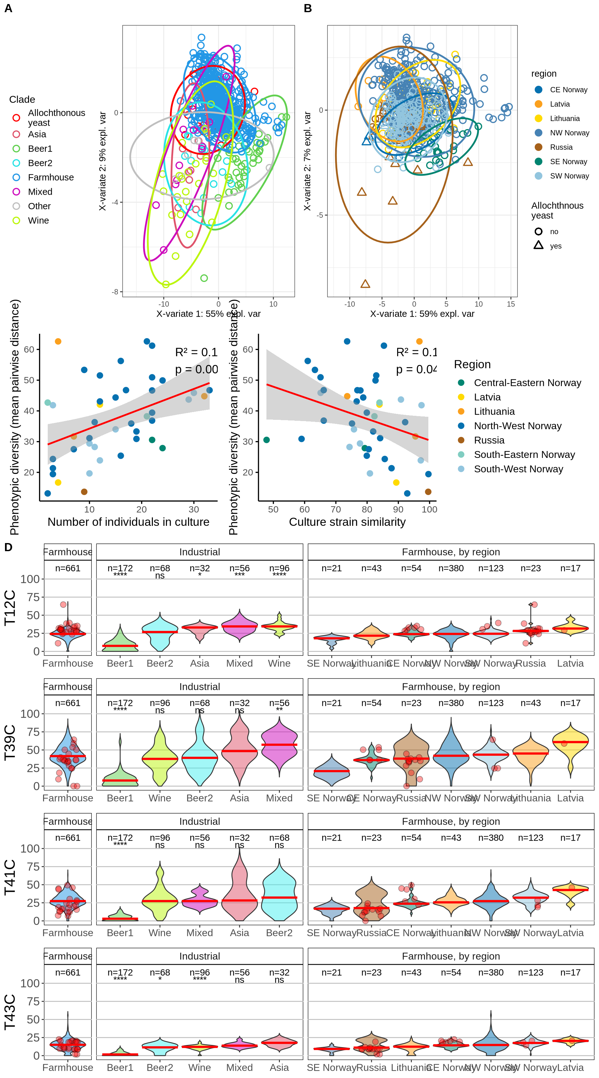
11 Figure 5
11.1 Figure 5 code
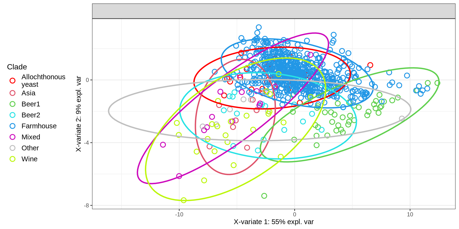
11.1.1 Panel A code
# import and prep data
raw_data = read.delim("./data/p02-05/grouped phenotype data with annotations.csv", sep = ",", header = TRUE)

raw_data = raw_data %>%
  dplyr::filter(group != "WL004") %>%
  dplyr::filter(group != "LA001")
raw_data$Industry = ifelse(
  raw_data$region %in% c("South-West Norway", "Lithuania", "North-West Norway", "Russia",
                         "Central-Eastern Norway", "Latvia", "South-Eastern Norway"),
  "Farmhouse",
  raw_data$region
)
raw_data$Industry = ifelse(
  raw_data$Outside == "yes",
  "Allochthonous\nyeast",
  raw_data$Industry
)
raw_data$region = ifelse(
  raw_data$Industry == "Farmhouse",
  raw_data$region,
  "NA"
)

raw_data$region = ifelse(
  raw_data$culture %in% c("7", "38"),
  "South-West Norway",
  ifelse(
    raw_data$culture == "40",
    "Russia",
    ifelse(
      raw_data$culture == "45",
      "Latvia",
      ifelse(
        raw_data$culture == "57",
        "Central-Eastern Norway",
        raw_data$region
      )
    )
  )
)


raw_data = raw_data %>%
  dplyr::mutate(region = dplyr::case_when(
    region == "South-West Norway" ~ "SW Norway",
    region == "North-West Norway" ~ "NW Norway",
    region == "Central-Eastern Norway" ~ "CE Norway",
    region == "South-Eastern Norway" ~ "SE Norway",
    .default = as.character(region)
  ))

metadata = raw_data %>%
  dplyr::select(c("group", "culture", "region", "Industry", "Outside", "method"))
rownames(metadata) = metadata$group

rownames(raw_data) = raw_data$group
counts = raw_data %>%
  dplyr::select(-c("group", "culture", "region", "Industry", "Outside", "method"))

# import final clade list
final_clades = read.table(
  "data/p02-05/final_clades_for_pub.txt",
  sep = "\t",
  header = TRUE,
  stringsAsFactors = FALSE
)
# replace
for(i in 1:nrow(final_clades)){

  strain = final_clades[i, "Strain"]
  clade = final_clades[i, "Clade"]
  metadata[which(metadata$group == strain), "Industry"] = clade

}
metadata$Industry = ifelse(metadata$Industry == "Beer", "Beer2", metadata$Industry)
metadata$Industry = ifelse(metadata$group == "BI001", "Asia", metadata$Industry)
metadata$Industry = ifelse(metadata$group == "BR003", "Mixed", metadata$Industry)
metadata$Industry = ifelse(metadata$group == "BI002", "Other", metadata$Industry)
metadata$Industry = ifelse(metadata$group == "BI004", "Asia", metadata$Industry)
metadata$Industry = ifelse(metadata$group == "BI005", "Other", metadata$Industry)


## background: no farmhouse
metadata_no_farm = metadata[which(metadata$Industry != "Farmhouse"), ]
counts_no_farm = counts[which(rownames(counts) %in% metadata_no_farm$group), ]

## farmhouse focus
metadata_farm_only = metadata[which(metadata$Industry %in% c("Farmhouse", "Allochthonous\nyeast")), ]
colnames(metadata_farm_only)[5] = "Allochthonous"
metadata_farm_only$Allochthonous = ifelse(metadata_farm_only$Allochthonous == "yes", "yes", "no")
counts_farm_only = counts[which(rownames(counts) %in% metadata_farm_only$group), ]


# sPLS-DA
counts_splsda = sapply(
  counts,
  function(counts) (counts-mean(counts))/stats::sd(counts)
)

# initial sPLS_DA
initial_splsda = mixOmics::splsda(
  counts_splsda,
  factor(metadata$Industry),
  ncomp = 10
) # set ncomp to 10 for performance assessment later

metadata$mock = "mock"
p_all_spls = mixOmics::plotIndiv(
  initial_splsda,
  comp = c(1, 2),
  group = factor(metadata$Industry),
  pch = factor(metadata$mock),
  ind.names = FALSE,
  ellipse = TRUE,
  legend = TRUE,
  legend.position = "left",
  legend.title = "Clade",
  title = "",
  col = c("red", "#df536b", "#61d04f", "#28e2e5", "#2297e6", "#cd0bbc", "grey75", "#bcf60c")
)
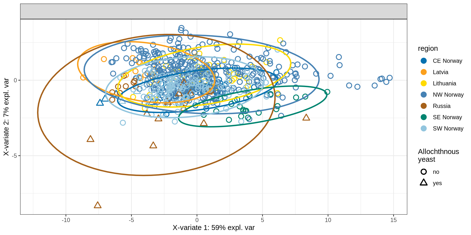
11.1.2 Panel B code
# initial sPLS_DA
initial_splsda = mixOmics::splsda(
  counts_farm_only,
  factor(metadata_farm_only$region),
  ncomp = 10
) # set ncomp to 10 for performance assessment later

p_farm_spls = mixOmics::plotIndiv(
  initial_splsda,
  comp = c(1, 2),
  group = factor(metadata_farm_only$region),
  pch = factor(metadata_farm_only$Allochthonous),
  ind.names = FALSE,
  ellipse = TRUE,
  legend = TRUE,
  legend.position = "left",
  legend.title = "region",
  legend.title.pch = "Allochthnous\nyeast",
  title = "",
  col = c('#0571B0', '#FBA01D',"#FFDA00", "steelblue", '#A6611A',"#008470",'#92C5DE')
)
11.1.3 Panel C code
# Load the dataset
mydata <- read.csv('./data/p02-05/grouped phenotype data with annotations.csv')

# Define region colors
RegionColors <- c(
  'North-West Norway' = '#0571B0',
  'South-West Norway' = '#92C5DE',
  'Central-Eastern Norway' = '#018571',
  'South-Eastern Norway' = '#80CDC1',
  'Latvia' = '#FFDA00',
  'Lithuania' = '#FBA01D',
  'Russia' = '#A6611A',
  'Beer' = '#FF0000',
  'Wine' = 'limegreen',
  'Outside' = '#000000'  # Black for the Outside group
)

# Create a new grouping variable:
# - "Outside" if Outside == "yes"
# - culture if available; otherwise, use region
mydata$grouping <- ifelse(
  mydata$Outside == "yes", "Outside",
  ifelse(is.na(mydata$culture), mydata$region, as.character(mydata$culture))
)

# Reorder the grouping factor with "Outside" first, then by region order
group_levels <- c("Outside", unique(mydata$grouping[mydata$grouping != "Outside"][order(mydata$region)]))
mydata$grouping <- factor(mydata$grouping, levels = group_levels)

# Select phenotypic data columns
phenotypic_data <- mydata %>% dplyr::select(Biggy:T43C)

# Calculate mean pairwise distance (multivariate diversity) per group
groupwise_distance <- mydata %>%
  dplyr::group_by(grouping) %>%
  dplyr::summarise(
    Mean_Pairwise_Distance = mean(
      vegdist(phenotypic_data[cur_group_rows(), ], method = "euclidean"),
      na.rm = TRUE
    ),
    n_individuals = n()
  )

# Combine the diversity metrics with region information
total_diversity <- groupwise_distance %>%
  left_join(mydata %>% dplyr::select(grouping, region) %>% distinct(), by = "grouping")

# (Optional) Check the diversity summary
print(total_diversity)
# A tibble: 55 × 4
grouping Mean_Pairwise_Distance n_individuals region
<fct> <dbl> <int> <chr>
1 Outside 66.8 24 Russia
2 Outside 66.8 24 South-West Norway
3 Outside 66.8 24 Latvia
4 Outside 66.8 24 South-Eastern Norway
5 Wild 56.3 4 Wild
6 Beer 105. 72 Beer
7 Wine 72.1 18 Wine
8 Spirits 69.5 6 Spirits
9 Bread 80.8 4 Bread
10 Sake 55.6 7 Sake
# ℹ 45 more rows# Remove specific rows if needed
total_diversity <- total_diversity[-c(1:10, 54:55), ]
# Test correlation between Mean Pairwise Distance and Number of Individuals
cor_test_distance <- cor.test(total_diversity$n_individuals, total_diversity$Mean_Pairwise_Distance, method = "pearson")
print(cor_test_distance)
    Pearson's product-moment correlation

data:  total_diversity$n_individuals and total_diversity$Mean_Pairwise_Distance
t = 3.0334, df = 41, p-value = 0.004183
alternative hypothesis: true correlation is not equal to 0
95 percent confidence interval:
 0.1466415 0.6454742
sample estimates:
      cor
0.4281293
# Extract correlation results for annotation
r_squared <- round(cor_test_distance$estimate^2, 2)
p_value <- signif(cor_test_distance$p.value, 3)
# Plot: Mean Pairwise Distance vs. Number of Individuals (colored by Region)
# Remove the legend from this plot since the color scheme is shared.
p_diversity_individuals <- ggplot(total_diversity, aes(x = n_individuals, y = Mean_Pairwise_Distance, color = region)) +
geom_point(size = 3) +
geom_smooth(method = "lm", color = "red", se = TRUE) +
scale_color_manual(values = RegionColors) +
labs(
x = "Number of individuals in culture",
y = "Phenotypic diversity\n(mean pairwise distance)"
) +
theme_classic(base_size = 14) +
theme(
legend.position = "none",
axis.line.x = element_line(color = "black"),
axis.line.y = element_line(color = "black"),
axis.ticks = element_line(color = "black")
) +
annotate("text",
x = max(total_diversity$n_individuals) * 0.8,
y = max(total_diversity$Mean_Pairwise_Distance) * 0.9,
label = paste0("R² = ", r_squared, "\np = ", p_value),
size = 5, hjust = 0)11.1.4 Panel D code
pheno_list = c(
  #"Biggy",
  "T12C",
  "T39C",
  "T41C",
  "T43C"
  #"T37C",
  #"EtOH_12",
  #"CuSO4_0.1",
  #"EtOH_10"
)

counts_long1 = counts %>%
  dplyr::mutate(group = rownames(counts)) %>%
  dplyr::left_join(metadata, by = "group") %>%
  reshape2::melt() %>%
  dplyr::filter(Industry %in% c("Farmhouse", "Allochthonous\nyeast")) %>%
  dplyr::filter(variable %in% pheno_list)
counts_long1$category = counts_long1$region
counts_long1$Industry = "Farmhouse"

counts_long2 = counts %>%
  dplyr::mutate(group = rownames(counts)) %>%
  dplyr::left_join(metadata, by = "group") %>%
  reshape2::melt() %>%
  dplyr::filter(variable %in% pheno_list)
counts_long2$category = ifelse(
  counts_long2$Industry %in% c("Farmhouse", "Allochthonous\nyeast"),
  "Farmhouse",
  counts_long2$Industry
)
counts_long2$region = counts_long2$category

counts_long3 = rbind(counts_long1, counts_long2)%>%
  dplyr::filter(region != "Other")
counts_long3$category = ifelse(
  counts_long3$category == "Allochthonous\nyeast", "Farmhouse", counts_long3$category
)
# counts_long3$region = ifelse(
#   is.na(counts_long3$region),
#   counts_long3$category,
#   counts_long3$region
# )

counts_long3$region = factor(
  counts_long3$region,
  levels = c(
    "SW Norway", "Lithuania", "NW Norway", "Russia",
    "CE Norway", "Latvia", "SE Norway",
    "Farmhouse", "Asia", "Beer1", "Beer2", "Mixed", "Wine"
    )
)

counts_long3$facet_factor = ifelse(
  counts_long3$region %in% c("SW Norway", "Lithuania", "NW Norway", "Russia",
                             "CE Norway", "Latvia", "SE Norway"),
  "Farmhouse, by region",
  ifelse(
    counts_long3$region %in% c("Asia", "Beer1", "Beer2", "Mixed", "Wine"),
    "Industrial",
    "Farmhouse"
  )
) %>% factor(
  levels = c("Farmhouse", "Industrial", "Farmhouse, by region")
)


text_annot = matrix(nrow = 13, ncol = 3) %>% data.frame
colnames(text_annot) = c("category", "facet_factor", "value")
text_annot$category = c(
  "Farmhouse",
  "CE Norway", "Latvia", "Lithuania", "NW Norway", "Russia", "SE Norway", "SW Norway",
  "Asia", "Beer1", "Beer2", "Mixed", "Wine"
)
text_annot$facet_factor = c(
  "Farmhouse",
  rep("Farmhouse, by region", 7),
  rep("Industrial", 5)
)
text_annot$value = c(
  661,
  54, 17, 43, 380, 23, 21, 123,
  32, 172, 68, 56, 96
)


color_annot = c(
  '#df536b', # Asia
  '#61d04f', # Beer1
  '#46f0f0', # Beer2
  "#008470", # CE Norway
  '#2297e6', # Farmhouse
  "#FFDA00", # Latvia
  '#FBA01D', # Lithuania
  '#cd0bbc', # Mixed
  '#0571B0', # NW Norway
  '#A6611A', # Russia
  "steelblue", # SE Norway
  '#92C5DE', # SW Norway
  '#bcf60c' # wine
)
color_annot = stats::setNames(
  color_annot,
  counts_long3$category %>% factor() %>% levels()
)


p_violins_final = list()

for(k in 1:length(pheno_list)){

  my_pheno = pheno_list[[k]]
  tmp_df = counts_long3 %>% dplyr::filter(variable == my_pheno)

  tests_pheno = tmp_df %>%
    dplyr::filter(facet_factor %in% c("Farmhouse", "Industrial")) %>%
    rstatix::t_test(value ~ Industry, ref.group = "Farmhouse")
  tests_pheno_annot = matrix(nrow = 5, ncol = 3) %>% data.frame
  colnames(tests_pheno_annot) = c("category", "facet_factor", "value")
  tests_pheno_annot$category = c("Asia", "Beer1", "Beer2", "Mixed", "Wine")
  tests_pheno_annot$facet_factor = c(rep("Industrial", 5))
  tests_pheno_annot$value = c(
    tests_pheno[2, "p.adj.signif"], tests_pheno[3, "p.adj.signif"], tests_pheno[4, "p.adj.signif"],
    tests_pheno[5, "p.adj.signif"], tests_pheno[6, "p.adj.signif"]
  )

  p_violins_final[[k]] = ggplot(tmp_df,
                                aes(x = forcats::fct_reorder(category, value, median),
                                    y = value)) +
    geom_violin(aes(fill = category),
                alpha = 0.5,
                scale = "width",
                trim = FALSE) +
    geom_point(data = tmp_df %>% dplyr::filter(Outside == "yes"),
               aes(x = category, y = value), fill = "red",
               position = position_jitter(width = 0.25),
               shape = 21,
               alpha = 0.375,
               size = 3) +
    geom_text(data = text_annot,
              aes(x = category, y = 115, label = paste0("n=", as.character(value)))) +
    geom_text(data = tests_pheno_annot,
              aes(x = category, y = 105, label = as.character(value))) +
    stat_summary(fun = "median", colour = "red", geom = "crossbar") +
    facet_grid(~ factor(facet_factor, levels = c("Farmhouse", "Industrial", "Farmhouse, by region")), scales = "free_x", space = "free") +
    scale_y_continuous(breaks = c(0, 25, 50, 75, 100), limits = c(0, 120), ) +
    scale_fill_manual(values = color_annot) +
    scale_x_discrete(labels = function(x) stringr::str_wrap(x, width = 10)) +
    labs(y = my_pheno) +
    theme(title = element_blank(),
          axis.text.x = element_text(size = 12),
          axis.text.y = element_text(size = 14),
          axis.title.x = element_blank(),
          axis.title.y = element_text(size = 18),
          legend.position = "none",
          panel.background = element_rect(colour = "black", fill = NA),
          panel.grid.major.x = element_blank(),
          panel.grid.minor.x = element_blank(),
          panel.grid.major.y = element_line(colour = "grey75"),
          panel.grid.minor.y = element_blank(),
          strip.background = element_rect(colour = "black", fill = NA),
          strip.text = element_text(size = 12))

}
11.1.5 Merge
final_plot = cowplot::plot_grid(
  cowplot::plot_grid(
    p_all_spls, p_farm_spls, p_diversity_individuals,
    nrow = 1,
    rel_widths = c(1, 1, 1),
    labels = c("A", "B", "C")
  ),
  cowplot::plot_grid(
    p_violins_final[[1]], p_violins_final[[2]], p_violins_final[[3]],
    p_violins_final[[4]],
    ncol = 1,
    labels = c("D", NA, NA, NA)
  ),
  nrow = 2,
  rel_heights = c(1.5, 2.5)
)
11.2 Figure 5 plot
11.3 Session Information
Note
R version 4.3.3 (2024-02-29)
Platform: x86_64-pc-linux-gnu (64-bit)
Running under: Ubuntu 24.04.3 LTS

Matrix products: default
BLAS:   /usr/lib/x86_64-linux-gnu/blas/libblas.so.3.12.0
LAPACK: /usr/lib/x86_64-linux-gnu/lapack/liblapack.so.3.12.0

locale:
 [1] LC_CTYPE=en_US.UTF-8    LC_NUMERIC=C            LC_TIME=C
 [4] LC_COLLATE=en_US.UTF-8  LC_MONETARY=C           LC_MESSAGES=en_US.UTF-8
 [7] LC_PAPER=C              LC_NAME=C               LC_ADDRESS=C
[10] LC_TELEPHONE=C          LC_MEASUREMENT=C        LC_IDENTIFICATION=C

time zone: Europe/Brussels
tzcode source: system (glibc)

attached base packages:
[1] stats     graphics  grDevices utils     datasets  methods   base

other attached packages:
 [1] vegan_2.7-1        permute_0.9-8      umap_0.2.10.0      RColorBrewer_1.1-3
 [5] PCAtools_2.14.0    patchwork_1.3.1    mixOmics_6.26.0    lattice_0.22-5
 [9] MASS_7.3-60.0.1    ggrepel_0.9.6      ggplot2_3.5.2      forcats_1.0.0
[13] dplyr_1.1.4

loaded via a namespace (and not attached):
 [1] tidyselect_1.2.1          farver_2.1.2
 [3] fastmap_1.2.0             digest_0.6.37
 [5] rsvd_1.0.5                lifecycle_1.0.4
 [7] cluster_2.1.6             magrittr_2.0.3
 [9] compiler_4.3.3            rlang_1.1.6
[11] tools_4.3.3               utf8_1.2.6
[13] igraph_2.1.4              yaml_2.3.10
[15] knitr_1.50                labeling_0.4.3
[17] askpass_1.2.1             S4Arrays_1.2.1
[19] dqrng_0.4.1               rARPACK_0.11-0
[21] htmlwidgets_1.6.4         reticulate_1.43.0
[23] DelayedArray_0.28.0       plyr_1.8.9
[25] abind_1.4-8               BiocParallel_1.36.0
[27] withr_3.0.2               purrr_1.1.0
[29] BiocGenerics_0.48.1       grid_4.3.3
[31] stats4_4.3.3              beachmat_2.18.1
[33] scales_1.4.0              dichromat_2.0-0.1
[35] cli_3.6.5                 ellipse_0.5.0
[37] rmarkdown_2.29            crayon_1.5.3
[39] generics_0.1.4            RSpectra_0.16-2
[41] reshape2_1.4.4            DelayedMatrixStats_1.24.0
[43] stringr_1.5.1             splines_4.3.3
[45] zlibbioc_1.48.2           parallel_4.3.3
[47] XVector_0.42.0            matrixStats_1.5.0
[49] vctrs_0.6.5               Matrix_1.6-5
[51] carData_3.0-5             jsonlite_2.0.0
[53] car_3.1-3                 BiocSingular_1.18.0
[55] IRanges_2.36.0            S4Vectors_0.40.2
[57] rstatix_0.7.2             Formula_1.2-5
[59] irlba_2.3.5.1             tidyr_1.3.1
[61] glue_1.8.0                codetools_0.2-19
[63] cowplot_1.2.0             stringi_1.8.7
[65] gtable_0.3.6              ScaledMatrix_1.10.0
[67] tibble_3.3.0              pillar_1.11.0
[69] htmltools_0.5.8.1         openssl_2.3.3
[71] R6_2.6.1                  sparseMatrixStats_1.14.0
[73] evaluate_1.0.4            backports_1.5.0
[75] png_0.1-8                 broom_1.0.9
[77] corpcor_1.6.10            Rcpp_1.1.0
[79] nlme_3.1-164              gridExtra_2.3
[81] SparseArray_1.2.4         mgcv_1.9-1
[83] xfun_0.52                 MatrixGenerics_1.14.0
[85] pkgconfig_2.0.3